eric melski's blog.melski.net

The Twelve Days of Christmas, GNU make style

Well, it’s Christmas Day in the States today, and while we’re all recovering from the gift-opening festivities, I thought this would be the perfect time for a bit of fun with GNU make. And what better subject matter than the classic Christmas carol “The Twelve Days of Christmas”? Its repetitive structure is perfect for demonstrating how to use several of GNU make’s built-in functions for iteration, selection and sorting. This simple makefile prints the complete lyrics to the song:

1
2
3
4
5
6
7
8
9
10
11
12
13
14
15
16
17
18
19
20
21
22
23
24
25

L01=Twelve drummers drumming,
L02=Eleven pipers piping,
L03=Ten lords-a-leaping,
L04=Nine ladies dancing,
L05=Eight maids-a-milking,
L06=Seven swans-a-swimming,
L07=Six geese-a-laying,
L08=Five golden rings,
L09=Four calling birds,
L10=Three french hens,
L11=Two turtle doves, and
L12=A partridge in a pear tree!
LINES=12 11 10 09 08 07 06 05 04 03 02 01
DAYS=twelfth eleventh tenth ninth \
	eighth seventh sixth fifth \
	fourth third second first
 
$(foreach n,$(LINES),\
	$(if $(X),$(info ),$(eval X=X))\
	$(info On the $(word $n,$(DAYS)) day of Christmas,)\
	$(info my true love gave to me)\
	$(foreach line,$(wordlist $n,12,$(sort $(LINES))),\
		$(info $(L$(line)))))
 
all: ; @:

By count, most of the lines here just declare variables, one for each item mentioned in the song. Note how the items are ordered: the last item added is given the lowest index. That means that to construct each verse we simply enumerate every item in the list, in order, starting with the new item in each verse.

Line 18 is where the real meat of the makefile begins. Here we use GNU make’s foreach function to iterate through the verses. $(foreach) takes three arguments: a name for the iteration variable, a space-separated list of words to assign to the iteration variable in turn, and a body of text to expand repeatedly, once for each word in the list. Here, the list of words is given by LINES, which lists the starting line for each verse, in order — that is, the first verse starts from line 12, the second from line 11, etc. The text to expand on each iteration is all the text on lines 19-23 of the makefile — note the use of backslashes to continue each line to the next.

Line 19 uses several functions to print a blank line before starting the next verse, if we’ve printed a verse already: the $(if) function, which expands its second argument if its first argument is non-empty, and its third argument if its first argument is empty; the $(info) function to print a blank line; and the $(eval) function to set the flag variable. The first time this line is expanded, X does not exist, so it expands to an empty string and the $(if) picks the “else” branch. After that, X has a value, so the $(if) picks the “then” branch.

Lines 20 and 21 again use $(info) to print output — this time the prelude for the verse, like “On the first day of Christmas, my true love gave to me”. The ordinal for each day is pulled from DAYS using the $(word) function, which extracts a specified word, given by its first argument, from the space-separated list given as its second argument. Here we’re using n, the iteration variable from our initial $(foreach) as the selector for $(word).

Line 22 uses $(foreach) again, this time to iterate through the lines in the current verse. We use line as the iteration variable. The list of words is given again by LINES except now we’re using $(sort) to reverse the order, and $(wordlist) to select a subset of the lines. $(wordlist) takes three arguments: the index of the first word in the list to select, the index of the last word to select, and a space-separated list of words to select from. The indices are one-based, not zero-based, and $(wordlist) returns all the words in the given range. The body of this $(foreach) is just line 23, which uses $(info) once more to print the current line of the current verse.

Line 25 has the last bit of funny business in this makefile. We have to include a make rule in the makefile, or GNU make will complain *** No targets. Stop. after printing the lyrics. If we simply declare a rule with no commands, like all:, GNU make will complain Nothing to be done for `all’.. Therefore, we define a rule with a single “no-op” command that uses the bash built-in “:” to do nothing, combined with GNU make’s @ prefix to suppress printing the command itself.

And that’s it! Now you’ve got some experience with several of the built-in functions in GNU make — not bad for a Christmas day lark:

$(eval) for dynamic interpretation of text as makefile content
$(foreach), for iteration
$(if), for conditional expansion
$(info), for printing output
$(sort), for sorting a list
$(word), for selecting a single word from a list
$(wordlist), for selecting a range of words from a list

Now — where’s that figgy pudding? Merry Christmas!

UPDATE: SCons is Still Really Slow

A while back I posted a series of articles exploring the scalability of SCons, a popular Python-based build tool. In a nutshell, my experiments showed that SCons exhibits roughly quadratic growth in build runtimes as the number of targets increases:

Recently Dirk Baechle attempted to rebut my findings in an entry on the SCons wiki: Why SCons is not slow. I thought Dirk made some credible suggestions that could explain my results, and he did some smart things in his effort to invalidate my results. Unfortunately, his methods were flawed and his conclusions are invalid. My original results still stand: SCons really is slow. In the sections that follow I’ll share my own updated benchmarks and show where Dirk’s analysis went wrong.

Test setup

As before, I used genscons.pl to generate sample builds ranging from 2,000 to 50,000 targets. However, my test system was much beefier this time:

	2013	2010
OS	Linux Mint 14 (kernel version 3.5.0-17-generic)	RedHat Desktop 3 (kernel version 2.4.21-58.ELsmp)
CPU	Quad 1.7GHz Intel Core i7, hyperthreaded	Dual 2.4GHz Intel Xeon, hyperthreaded
RAM	16 GB	2 GB
HD	SSD	(unknown)
SCons	2.3.0	1.2.0.r3842
Python	2.7.3 (system default)	2.6.2

Before running the tests, I rebooted the system to ensure there were no rogue processes consuming memory or CPU. I also forced the CPU cores into “performance” mode to ensure that they ran at their full 1.7GHz speed, rather than at the lower 933MHz they switch to when idle.

Revisiting the original benchmark

I think Dirk had two credible theories to explain the results I obtained in my original tests. First, Dirk wondered if those results may have been the result of virtual memory swapping — my original test system had relatively little RAM, and SCons itself uses a lot of memory. It’s plausible that physical memory was exhausted, forcing the OS to swap memory to disk. As Dirk said, “this would explain the increase of build times” — you bet it would! I don’t remember seeing any indication of memory swapping when I ran these tests originally, but to be honest it was nearly 4 years ago and perhaps my memory is not reliable. To eliminate this possibility, I ran the tests on a system with 16 GB RAM this time. During the tests I ran vmstat 5, which collects memory and swap usage information at five second intervals, and captured the result in a log.

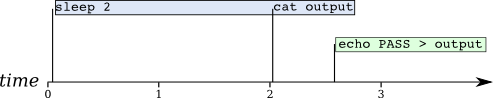
Next, he suggested that I skewed the results by directing SCons to inherit the ambient environment, rather than using SCons’ default “sanitized” environment. That is, he felt I should have used env = Environment() rather than env = Environment(ENV = os.environ). To ensure that this was not a factor, I modified the tests so that they did not inherit the environment. At the same time, I substituted echo for the compiler and other commands, in order to make the tests faster. Besides, I’m not interested in benchmarking the compiler — just SCons! Here’s what my Environment declaration looks like now:

env = Environment(CC = 'echo', AR = 'echo', RANLIB = 'echo')

With these changes in place I reran my benchmarks. As expected, there was no change in the outcome. There is no doubt: SCons does not scale linearly. Instead the growth is polynomial, following an n^1.85 curve. And thanks to the the vmstat output we can be certain that there was absolutely no swapping affecting the benchmarks. Here’s a graph of the results, including an n^1.85 curve for comparison — notice that you can barely see that curve because it matches the observed data so well!

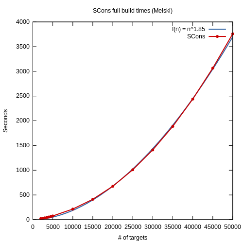
For comparison, I used the SCons build log to make a shell script that executes the same series of echo commands. At 50,000 targets, the shell script ran in 1.097s. You read that right: 1.097s. Granted, the shell script doesn’t do stuff like up-to-date checks, etc., but still — of the 3,759s average SCons runtime, 3,758s — 99.97% — is SCons overhead.

I also created a non-recursive Makefile that “builds” the same targets with the same echo commands. This is a more realistic comparison to SCons — after all, nobody would dream of actually controlling a build with a straight-line shell script, but lots of people would use GNU make to do it. With 50,000 targets, GNU make ran for 82.469s — more than 45 times faster than SCons.

What is linear scaling?

If the performance problems are so obvious, why did Dirk fail to see them? Here’s a graph made from his test results:

Dirk says that this demonstrates “SCons’ linear scaling”. I find this statement baffling, because his data clearly shows that SCons does not scale linearly. It’s simple, really: linear scaling just means that the build time increases by the same amount for each new target you add, regardless of how many targets you already have. Put another way, it means that the difference in build time between 1,000 targets and 2,000 targets is exactly the same as the difference between 10,000 and 11,000 targets, or between 30,000 and 31,000 targets. Or, put yet another way, it means that when you plot the build time versus the number of targets, you should get a straight line with no change in slope at any point. Now you tell me: does that describe Dirk’s graph?

Here’s another version of that graph, this time augmented with a couple additional lines that show what the plot would look like if SCons were truly scaling linearly. The first projection is based on the original graph from 2,500 to 4,500 targets — that is, if we assume that SCons scales linearly and that the increase in build time between 2,500 and 4,500 targets is representative of the cost to add 2,000 more targets, then this line shows us how we should expect the build time to increase. Similarly, the second projection is based on the original graph between 4,500 and 8,500 targets. You can easily see that the actual data does not match either projection. Furthermore you can see that the slope of these projections is increasing:

This shows the importance of testing at large scale when you’re trying to characterize the scalability of a system from empirical data. It can be difficult to differentiate polynomial from logarithmic or linear at low scales, especially once you incorporate the constant factors — polynomial algorithms can sometimes even give better absolute performance for small inputs than linear algorithms! It’s not until you plot enough data points at large enough values, as I’ve done, that it becomes easy to see and identify the curve.

What does profiling tell us?

Next, Dirk reran some of his tests under a profiler, on the very reasonable assumption that if there was a performance problem to be found, it would manifest in the profiling data — surely at least one function would demonstrate a larger-than-expected growth in runtime. Dirk only shared profiling data for two runs, both incremental builds, at 8,500 and 16,500 targets. That’s unfortunate for a couple reasons. First, the performance problem is less apparent on incremental builds than on full builds. Second, with only two datapoints it is literally not possible to determine whether growth is linear or polynomial. The results of Dirk’s profiling was negative: he found no “significant difference or increase” in any function.

Fortunately it’s easy to run this experiment myself. Dirk used cProfile, which is built-in to Python. To profile a Python script you can inject cProfile from the command-line, like this: python -m cProfile scons. Just before Python exits, cProfile dumps timing data for every function invoked during the run. I ran several full builds with the profiler enabled, from 2,000 to 20,000 targets. Then I sorted the profiling data by function internal time (time spent in the function exclusively, not in its descendents). In every run, the same two functions appeared at the top of the list: posix.waitpid and posix.fork. To be honest this was a surprise to me — previously I believed the problem was in SCons’ Taskmaster implementation. But I can’t really argue with the data. It makes sense that SCons would spend most of its time running and waiting for child processes to execute, and even that the amount of time spent in these functions would increase as the number of child processes increases. But look at the growth in runtimes in these two functions:

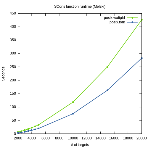
Like the overall build time, these curves are obviously non-linear. Armed with this knowledge, I went back to Dirk’s profiling data. To my surprise, posix.waitpid and posix.fork don’t even appear in Dirk’s data. On closer inspection, his data seems to include only a subset of all functions — about 600 functions, whereas my profiling data contains more than 1,500. I cannot explain this — perhaps Dirk filtered the results to exclude functions that are part of the Python library, assuming that the problem must be in SCons’ own code rather than in the library on which it is built.

This demonstrates a second fundamental principle of performance analysis: make sure that you consider all the data. Programmers’ intuition about performance problems is notoriously bad — even mine! — which is why it’s important to measure before acting. But measuring won’t help if you’re missing critical data or if you discard part of the data before doing any analysis.

Conclusions

On the surface, performance analysis seems like it should be simple: start a timer, run some code, stop the timer. Done correctly, performance analysis can illuminate the dark corners of your application’s performance. Done incorrectly — and there are many ways to do it incorrectly — it can lead you on a wild goose chase and cause you to squander resources fixing the wrong problems.

Dirk Baechle had good intentions when he set out to analyze SCons performance, but he made some mistakes in his process that led him to an erroneous conclusion. First, he didn’t run enough large-scale tests to really see the performance problem. Second, he filtered his experimental data in a way that obscured the existence of the problem. But perhaps his worst mistake was to start with a conclusion — that there is no performance problem — and then look for data to support it, rather than starting with the data and letting it impartially guide him to an evidence-based conclusion.

To me the evidence seems indisputable: SCons exhibits roughly quadratic growth in runtimes as the number of build targets increases, rendering it unusable for large-scale software development (tens of thousands of build outputs). There is no evidence that this is a result of virtual memory swapping. Profiling suggests a possible pair of culprits in posix.waitpid and posix.fork. I leave it to Dirk and the SCons team to investigate further; in the meantime, you can find my test harness and test results in my GitHub repo. If you can see a flaw in my methodology, sound off in the comments!

Halloween 2013 haunted graveyard

I know it’s a bit late for a retrospective on my annual Halloween tradition — the haunted graveyard. But there were a couple additions this year that I thought were worth mentioning, and I have some really excellent photos thanks to the efforts of a good friend so I figured “Better late than never!” For those who haven’t seen my previous articles about the graveyard, let me offer a brief backstory:

After my wife and I inherited her mother’s house several years ago, it became our responsibility to host the annual family Halloween party. Originally the party was intended for my mother-in-law’s adult children and their spouses, but once they started having kids of their own, the party shifted gears. It’s been primarily targeted at the kids as long as I’ve been involved. One of the marquee attractions is the haunted graveyard, where our backyard is transformed from a normal suburban plot into a spooky graveyard replete with zombies, ghosts and other monsters. As the man of the house, and because I have a bit of a macabre streak, it falls to me to design and … execute … the decorations. Every year the graveyard gets a little bit more elaborate as I snatch up more characters at the post-Halloween sales and devise better layouts and designs for the graveyard.

As in previous years, I used a short two-foot tall wooden fence to establish a perimeter for the graveyard. This serves two purposes. First, it provides a pathway for visitors to follow, so they aren’t just meandering through the graveyard. That allows me to better control the experience and ensure that people don’t approach characters from the wrong side. Second, it gives a little protection to the characters, to discourage children from physically abusing the decorations. You can see the fencing here (as usual, click on any of these pictures for a larger version):

Along with the fence you can see one of the architectural improvements in the graveyard: a dividing wall down the middle of the area. This serves to block view of the characters on the second half of the graveyard when you are walking down the first half. I fashioned this out of several pieces of 1 inch PVC pipe and PVC pipe connectors at a total cost of about $20 at the local hardware store. PVC’s a great choice for this because it’s cheap, lightweight and easy to work with — all you need is a hacksaw. It’s also easy to setup and tear down. This diagram shows the dimensions and parts I used to build the frame:

The curtain is made from two black plastic tablecloths, the type you can find at a party supply store around Halloween time. The ends are folded over and stapled together to make sleeves into which the top and bottom PVC pipes can slide. I think the tablecloths cost about $8 each. To be honest the whole thing looks pretty cheap in the daylight, but once it gets dark it doesn’t matter. Next year I’ll probably blacken the PVC with some spraypaint. If I can find some cheap cloth, I’ll redo the curtains as well. If you do build something like this yourself, make sure that the feet are pretty wide, and put something heavy on each to hold it down. Otherwise one good gust of wind will knock your wall right over!

As for new characters this year, I have this creepy-as-hell “deady bear”. For such a small guy, he is surprisingly disturbing. When activated, his head turns side-to-side, one eyeball lights up, he stabs himself with a knife, and he makes seriously unsettling noises. Like most of the characters he’s sound activated:

I’ve also got this “zombie barrel”, who lights up, makes spooky sounds and rises up out of his barrel when activated. To be honest although he’s big and was expensive, it’s not one of my favorite characters. He’s difficult to setup, and he moves too slowly to be really scary:

Unfortunately I don’t have a picture of the third new character — this black jumping spider. This guy is great because he moves quickly, and he’s hard to see since he’s black and starts at ground level. It’s very startling — perfect for somebody coming around a corner.

Besides the partition and the new characters, there was one other upgrade that I’m really pleased with: the flying phantasm. I’ve actually had this character for a couple of years, but usually he just hangs “lifelessly” over the path:

This year I ran a 1/4 inch rope from my second-story roof to the fence at the edge of our property, then attached the ghost to a cheap pulley that I hung on the line:

Once the line was taut, the ghost could “fly” down the line across the pathway, low enough that his tattered robe would brush against the head and shoulders of anybody walking by. Triggering the ghost was about as low-tech as it gets: somebody would watch from a second floor window behind the ghost and release him at suitable moments; a bit of string tied to his back allowed my cohort to pull him back up in preparation for the next run. After dark, the flying phantasm was a huge hit, even scaring some of the adults who went through the graveyard! Here’s a video of the daytime test run; you can see where I’ve got a bit of extra rope tied around the line to serve as a stop so that he doesn’t go too far:

That’s about it for new features this year. Overall I think this goes down as another success, but there are some things I’d like to improve for next year:

Get more foot activation pads! I cannot stress enough how critical these are. The sound activation on most of these characters just does not work very well, especially when people are creeping silently through (because they are too scared to make much noise!). One trick though: make sure the pads are covered up, otherwise they are a huge tip off that something is coming!
Improve the lighting! I have simultaneously too much and not enough light. The colored floods I’ve been using are too bright, which makes things less scary. But they also don’t provide enough light in the right places. For example, it was hard to see the “deady bear”. Next year I’ll use dimmer bulbs, and maybe get some of those little “hockey puck” style LED lights to provide target “up lighting” for specific characters. I’d love to hang one dim, naked bulb over the whole scene as well, that could just swing back and forth slowly — I think that would be really creepy looking.
Don’t forget the soundtrack! I have one of those “scary halloween sounds” albums that I’ve played in the past to good effect. I completely forgot to set that up this year.

Hope you enjoyed this post mortem! To wrap up, here are some pictures of the graveyard after dark — credit goes to my good friend Tim Murphy, who took most of the pictures used in this post, and who was a tremendous help in setting up the graveyard. See you next Halloween!

The ElectricAccelerator 7.1 “Ship It!” Award

Well, it took a lot longer than I’d like, but at last I can reveal the Accelerator 7.1 “Ship It!” award. This is the fifth time I’ve commemorated our releases in this fashion, which I think is pretty cool itself.

Since this release again focused on performance, I picked a daring old-timey airplane pilot — the sort of guy you might have found behind the controls of a Sopwith Camel, with a maximum speed of about 115mph. Here’s the trading card that accompanied the figure:

Accelerator 7.1 “Ship It!” Card Front – click for larger version

Accelerator 7.1 “Ship It!” Card Back – click for larger version

I included release metrics again, but where the 7.0 card showed just 10 data points, the 7.1 card packs in a whopping 48 by including data for the 12 most recent releases across four categories;

Number of days in development.
JIRA issues closed.
Total KLOC. This metric gives the total size of the Accelerator code base in thousands of lines of code, as measured with the excellent Count Lines of Code utility by Al Danial. This measurement excludes comments and whitespace.
Change in KLOC. This is simply the arithmetic difference between the total KLOC for each release and its predecessor.

Again, my sincere gratitude goes to everybody on the Accelerator team. Well done and thank you!

What’s new in GNU make 4.0?

After a little bit more than three years, the 4.0 release of GNU make finally arrived in October. This release packs in a bunch of improvements across many functional areas including debuggability and extensibility. Here’s my take on the most interesting new features.

Output synchronization

For the majority of users the most exciting new feature is output synchronization. When enabled, output synchronization ensures that the output of each job is kept distinct, even when the build is run in parallel. This is a tremendous boon to anybody that’s had the misfortune of having to diagnose a failure in a parallel build. This simple Makefile will help demonstrate the feature:

1
2
3
4
5
6
7
8
9
10
11
12

all: a b c
a:
   @echo COMPILE a
   @sleep 1 && echo a, part 1
   @sleep 1 && echo a, part 2
   @sleep 2 && echo a, part 3
 
b c:
   @echo COMPILE $@
   @sleep 1 && echo $@, part 1
   @sleep 1 && echo $@, part 2
   @sleep 1 && echo $@, part 3

Now compare the output when run serially, when run in parallel, and when run in parallel with –output-sync=target:

Serial Parallel Parallel with –output-sync=target

$ gmake
COMPILE a
a, part 1
a, part 2
a, part 3
COMPILE b
b, part 1
b, part 2
b, part 3
COMPILE c
c, part 1
c, part 2
c, part 3

$ gmake -j 4
COMPILE a
COMPILE b
COMPILE c
b, part 1
a, part 1
c, part 1
b, part 2
a, part 2
c, part 2
b, part 3
c, part 3
a, part 3

$ gmake -j 4 --output-sync=target
COMPILE c
c, part 1
c, part 2
c, part 3
COMPILE b
b, part 1
b, part 2
b, part 3
COMPILE a
a, part 1
a, part 2
a, part 3

Here you see the classic problem with parallel gmake build output logs: the output from each target is mixed up with the output from other targets. With output synchronization, the output from each target is kept separate, not intermingled. Slick! The output doesn’t match that of the serial build, unfortunately, but this is still a huge step forward in usability.

The provenance of this feature is especially interesting, because the idea can be traced directly back to me — in 2009, I wrote an article for CM Crossroads called Descrambling Parallel Build Logs. That article inspired David Boyce to submit a patch to GNU make in 2011 which was the first iteration of the –output-sync feature.

GNU Guile integration

The next major addition in GNU make 4.0 is GNU Guile integration, which makes it possible to invoke Guile code directly from within a makefile, via a new $(guile) built-in function. Naturally, since Guile is a general-purpose, high-level programming language, this allows for far more sophisticated computation from directly within your makefiles. Here’s an example that uses Guile to compute Fibonacci numbers — contrast with my Fibonacci in pure GNU make:

1
2
3
4
5
6
7
8
9
10
11

define FIBDEF
(define (fibonacci x)
 (if (< x 2)
  x
  (+ (fibonacci (- x 1)) (fibonacci (- x 2)))))
#f
endef
$(guile $(FIBDEF))
 
%:
   @echo $(guile (fibonacci $@))

Obviously, having a more expressive programming language available in makefiles will make it possible to do a great deal more with your make-based builds than ever before. Unfortunately I think the GNU make maintainers made a couple mistakes with this feature which will limit its use in practice. First, Guile was a poor choice. Although it’s a perfectly capable programming language, it’s not well-known or in wide use compared to other languages that they might have chosen — although you can find Scheme on the TIOBE Index, Guile itself doesn’t show up, and even though it is the official extension language of the GNU project, fewer than 25 of the GNU project’s 350 packages use Guile. If the intent was to embed a language that would be usable by a large number of developers, Python seems like the no-brainer option. Barring that for any reason, Lua seems to be the de facto standard for embedded programming languages thanks to its small footprint and short learning curve. Guile is just some weird also-ran.

Second, the make/Guile integration seem a bit rough. The difficulty arises from the fact that Guile has a rich type system, while make does not — everything in make is a string. Consequently, to return values from Guile code to make they must be converted to a string representation. For many data types — numbers, symbols and of course strings themselves — the conversion is obvious, and reversible. But for some data types, this integration does a lossy conversion which makes it impossible to recover the original value. Specifically, the Guile value for false, #f, is converted to an empty string, rendering it indistinguishable from an actual empty string return value. In addition, nested lists are flattened, so that (a b (c d) e) becomes a b c d e. Of course, depending on how you intend to use the data, each of these may be the right conversion. But that choice should be left to the user, so that we can retain the additional information if desired.

Loadable objects

The last big new feature in GNU make 4.0 is the ability to dynamically load binary objects into GNU make at runtime. In a nutshell, that load of jargon means that it’s possible for you to add your own “built-in” functions to GNU make, without having to modify and recompile GNU make itself. For example, you might implement an $(md5sum) function to compute a checksum, rather than using $(shell md5sum). Since these functions are written in C/C++ they should have excellent performance, and of course they can access the full spectrum of system facilities — file I/O, sockets, pipes, even other third-party libraries. Here’s a simple extension that creates a $(fibonacci) built-in function:

#include <stdio.h>
#include <gnumake.h>

int plugin_is_GPL_compatible;

int fibonacci(int n)
{
    if (n < 2) {
        return n;
    }
    return fibonacci(n - 1) + fibonacci(n - 2);
}

char *gm_fibonacci(const char *nm, unsigned int argc, char **argv)
{
    char *buf  = gmk_alloc(33);
    snprintf(buf, 32, "%d", fibonacci(atoi(argv[0])));
    return buf;
}

int fibonacci_gmk_setup ()
{
    gmk_add_function ("fibonacci", gm_fibonacci, 1, 1, 0);
    return 1;
}

And here’s how you would use it in a makefile:

1
2
3

load ./fibonacci.so
%:
   @echo $(fibonacci $@)

I’m really excited about this feature. People have been asking for additional built-in functions for years — to handle arithmetic, file I/O, and other tasks — but for whatever reason the maintainers have been slow to respond. In theory, loadable modules will enable people to expand the set of built-in functions without requiring the approval or involvement of the core team. That’s great! I only wish that the maintainers had been more responsive when we invited them to collaborate on the design, so we might have come up with a design that would work with both GNU make and Electric Make, so that extension authors need only write one version of their code. Ah well — que sera, sera.

Other features

In addition to the major feature described above there are several other enhancements worth mentioning here:

::= assignment, equivalent to := assignment, added for POSIX compatibility.
!= assignment, which is basically a substitute for $(shell), added for BSD compatibility.
–trace command-line option, which causes GNU make to print commnds before execution, even if they would normally be suppressed by the @ prefix.
$(file …) built-in function, for writing text to a file.
GNU make development migrated from CVS to git.

You can find the full list of updates in the NEWS file in the GNU make source tree.

Looking ahead

It’s great to see continued innovation in GNU make. Remember, this is a tool that’s now 25 years old. How much of the software you wrote 25 years ago is still in use and still in active development? I’d like to offer a heartfelt congratulations to Paul Smith and the rest of the GNU make team for their accomplishments. I look forward to seeing what comes next!

What’s new in ElectricAccelerator 7.1

ElectricAccelerator 7.1 hit the streets a last month, on October 10, just six months after the 7.0 release in April. There are some really cool new features in this release, which picks up right where 7.0 left off by adding even more ground-breaking performance features: schedule optimization and Javadoc caching. Here’s a quick look at each.

Schedule Optimization

The idea behind schedule optimization is really simple: we can reduce overall build duration if we’re smarter about the order in which jobs are run. In essense, it’s about packing the jobs in tighter, eliminating idle time in the middle of the build and reducing the “ragged right edge”. Here’s a side-by-side comparison of the same build, first using normal scheduling and then using schedule optimization. You can easily see that schedule optimization made the second build faster — an 11% improvement in this small, real-world example:

Build using naive scheduling — click to view full size

Build using schedule optimization – click to view full size

If you study the two runs more closely, you can see how schedule optimization produced this improvement: key jobs, in particular the longest jobs, were started earlier. As a result, idle time in the middle of the build was reduced or eliminated entirely, and the right edge is much less uneven. But the best part? It’s completely automatic: all you have to do is run the build once for emake to learn its performance profile. Every subsequent build will leverage that data to improve build performance, almost like magic.

Not convinced? Here’s a look at the impact of schedule optimization on another, much bigger proprietary build (serial build time 18h25m). The build is already highly parallelizable and achieves an impressive 37.2x speedup with 48 agents — but schedule optimization can reduce the build duration by nearly 25% more, bringing to total speedup on 48 agents to an eye-popping 47.5x!

Build duration with naive and optimized scheduling

There’s another interesting angle to schedule optimization though. Most people will take the performance gains and use them to get a faster build on the same hardware. But you could go the other direction just as easily — keep the same build duration, but do it with dramatically less hardware. The following graph quantifies the savings, in terms of cores needed to achieve a particular build duration. Suppose we set a target build duration of 30 minutes. With naive scheduling, we’d need 48 agents to meet that target. With schedule optimization, we need only 38.

Resource requirements with naive and optimized scheduling – click for full size

I’m really excited about schedule optimization, because it’s one of those rare features that give you something for nothing. It’s also been a long time coming — the idea was originally conceived of over three years ago, and it’s only now that we were able to bring it to fruition.

Schedule optimization works with emake on all supported platforms, with all emulation modes. It is not currently available for use with electrify.

Javadoc caching

The second major feature in Accelerator 7.1 is Javadoc caching. Again, it’s a simple idea: think “ccache”, but for Javadoc instead of compiles. This is the next phase in the evolution of Accelerator’s output reuse initiative, which began in the 7.0 release with parse avoidance. Like any output reuse feature, Javadoc caching works by capturing the product of a Javadoc invocation and storing it in a cache indexed by a hash of the inputs used — including the Java files themselves, the environment variables, and the command-line. In subsequent builds, emake will check those inputs again and if it computes the same hash, emake will used the cached results instead of running Javadoc again. On big Javadoc jobs, this can produce significant savings. For example, in the Android “Jelly Bean” open-source build, the main Javadoc invocation usually takes about five minutes. With Javadoc caching in Accelerator 7.1, that job runs in only about one minute — an 80% reduction! In turn that gives us a full one minute reduction in the overall build time, dropping the build from 13 minutes to 12 — nearly a 10% improvement:

Uncached Javadoc job in Android build – click for full image

Cached Javadoc job in Android build - click for full build

Cached Javadoc job in Android build – click for full image

Javadoc caching is available on Solaris and Linux only in Accelerator 7.1.

Looking ahead

I hope you’re as excited about Accelerator 7.1 as I am — for the second time this year, we’re bringing revolutionary new performance features to the table. But of course our work is never done. We’ve been hard at work on the “buddy cluster” concept for the next release of Accelerator. Hopefully I’ll be able to share some screenshots of that here before the end of the year. We’re also exploring acceleration for Bitbake builds like the Yocto Project. And last, but certainly not least, we’ll soon start fleshing out the next phase of output reuse in Accelerator — caching compiler invocations. Stay tuned!

SPARK 2013 by the Numbers

A few weeks ago we wrapped up the sixth annual Electric Cloud Summit: SPARK 2013. This year’s event was hands down the best we’ve done, with more content, more speakers and more attendees than ever before. For the first time we had invited keynote speakers including agile development and continuous delivery luminaries like Jez Humble (who literally wrote the book on continuous delivery!) and Gene Kim. We also had live streaming so that people who couldn’t make it to the conference in person could still watch and listen to the keynote sessions — if you missed the conference, you can watch the recordings now, and I really recommend that you do.

As usual, I did some analysis of the event once the conference was over. Here are the results.

Registration and Attendance

Each year since its inception, the summit has set a new record for total registrations, and SPARK 2013 was no exception with 186 people signed up. But even more impressive is the record 168 attendees — those people that actually made it to the conference. That beats the previous high of 146 from 2011 and is a massive 33% increase from the 126 attendees in 2012:

But that’s not the end of the story on attendance this year, because for the first time we offered live streaming over the Internet. That added an impressive 84 additional “virtual” attendees to the keynote session, bringing the total to over 250 attendees.

I think three factors contributed to the high registration and the better-than-90% conversion rate. First, there’s no doubt that the list of keynote speakers helped attract people to the event:

Jez Humble, co-author of “Continuous Delivery”
Gary Gruver, co-author of “A Practical Approach to Large-Scale Agile Development”
Gene Kim, author of “The Phoenix Project”
Paul Rogers, Chief Development Office at General Electric

Second, this was the first time that the conference was open to the public rather than being exclusively for Electric Cloud customers. Finally, this was the first time that attendees paid to attend the conference — somewhat counter-intuitively, you can sometimes increase interest in an offering simply by charging more for it. I think this has to do with the perceived value of the offering: some people think, “If this is free, it must not be very good.” Plus, once you’ve paid for a conference, you’re more likely to attend because you don’t want your money to go to waste.

Repeat attendance

A solid 25% of the attendees in 2013 had attended at least one previous summit, slightly down from the percentage of repeat attendees in 2012, but in line with the historical average. Amazingly, three die-hard users have attended all six conferences!

Presentations

SPARK 2013 had about 20% more sessions than 2012, and again more of the content came from users and partners than in any previous year. Sadly I didn’t get a chance to see too many of the presentations since I was a presenter myself, but I did get to watch the keynotes at least. If you didn’t watch the SPARK 2013 keynotes yet, you really should. It’s OK, I’ll wait.

The 2013 conference had 35 sessions in total, spanning four days and three tracks, including all the keynotes, training and track sessions:

Origins

As usual, the majority of attendees were from the United States, but a respectable 10% braved international travel to attend in person:

Fourteen US states were represented — the exact number of states represented in 2012 and in 2011, but a different set from either of those years. If I didn’t know better I’d say this was evidence of some kind of conspiracy. As expected, most of the US attendees were from California, but about 20% were from other states:

Industries and Delegations

67 companies sent people to SPARK 2013, representing a broad array of industries. Some of those are the usual suspects, like software and telecommunications, but there are some surprises as well, like the 4 companies in the retail industry and the one in education. As they say, software is eating the world. Many companies sent only one representative, but just a bit more than half sent two or more. One large networking company sent fifteen people to SPARK 2013!

Rate of registration

Finally, here’s a look at the rate of registration in the weeks leading up to SPARK 2013. In 2012 I hypothesized that the relatively low attendance numbers were partly because promotional activity for the event didn’t really get started until about 9 weeks prior to the conference. I thought perhaps that was not enough lead time for people. But to my surprise, the same is true this year and yet we had significantly more registrations than in 2012. I still think we could get even more if we started promoting the event earlier, but obviously there’s more to the story than simply that. The good news is that the team behind SPARK 2013 is already planning for SPARK 2014, so hopefully next year we’ll see if I’m right.

Don’t miss SPARK 2014!

Overall I think SPARK 2013 represents a turning point in the evolution of the Electric Cloud Summit. In a way it’s like we’re finally “growing up”, going from a small, private event to a serious public conference. I can’t wait to see what SPARK 2014 looks like, and I hope you’ll all join me there next year!

The inverted parallel build bug

At some point most of you have encountered “the” parallel build problem: a build that works just fine when run serially, but breaks sometimes when run in parallel. You may have read my blog about how ElectricAccelerator automatically solves the classic parallel build problem. Recently I ran into the opposite problem in a customer’s build: a build that “works” when run in parallel, but breaks when run serially! If you’re lucky, this build defect will just cause occasional build failures. If you’re unlucky, it will silently corrupt your build output at random. With traditional GNU make this nasty bug is a nightmare to track down — if you even know that its present!

In contrast, the unique features in ElectricAccelerator make it trivial to find the defect — some might even say it’s fun (well, if you’re like me and you enjoy using powerful tools to do sophisticated analysis without breaking a sweat!). Read on to see how ElectricAccelerator makes it easy to diagnose and fix bugs in your build.

The inverted parallel build bug

Let’s start with a concrete example. Here’s a simple Makefile which (appears to) work when run in parallel, but which consistently fails serially:

1
2
3
4
5
6
7
8

all: reader writer
	
reader:
	sleep 2
	cat output
	
writer:
	echo PASS > output

Assuming that output does not exist, executing this makefile serially will always produce an error:

$ gmake
sleep 2
cat output
cat: output: No such file or directory
gmake: *** [reader] Error 1

But if you execute this makefile in parallel, it appears to work!:

$ gmake -j 2
sleep 2
echo PASS > output
cat output
PASS

If we visualize the execution of these commands it’s easy to see why the parallel build seems to work:

At the beginning of the build, both reader and writer are started, more-or-less at the same time, because we told gmake to run two jobs at a time. reader has two commands, which are executed serially according to the semantics of make. While the sleep 2 is executing, the echo command in writer runs and completes. When the cat command in reader starts, it succeeds because output is ready-to-go.

Parallel execution is no guarantee

Some people will look at that explanation and think “Got it — always run this thing in parallel and we’re good!” Of course, you can’t really be 100% sure that everybody will remember to run the makefile in parallel. But even if you could, there’s a flaw in that reasoning: basically, your build has a race condition, and there’s no guarantee that you’ll “win” the race every time. For example, if your build server is heavily loaded, the sequence of events might look like this instead:

Here, writer doesn’t get started until after the sleep command has finished — too late to save the cat command from failure.

Build failure is not the worst outcome

Before we move on to finding and fixing problems like this, let’s take a quick look at one more failure mode: incremental builds. In particular, check out what happens if output exists before the build starts, but with incorrect content (for example, stale data from an earlier build):

$ echo '*** FAIL ***' > output
$ gmake
sleep 2
cat output
*** FAIL ***
echo PASS > output
$ echo $?
0

That’s right — the build “succeeded”, because it produced no error messages and exited with a zero exit code. And yet, it produced completely bogus output. Ouch!

Somebody save me!

If you’re using ordinary GNU make, you’re in for a world of hurt with a problem like this. First, the only way to consistently reproduce the problem is to run the entire build serially — of course that probably takes a long time, or you wouldn’t have been using parallel builds in the first place. Second, there are no diagnostics built into gmake that could help you identify which job produces output. One option is to use strace to monitor filesystem accesses, but that will generate a mountain of data in a not-very-usable format. Plus, it imposes a substantial performance penalty — on top of the hit you’d already take for running the build serially. Yuck!

If you’re using Electric Make, this problem is embarrassingly easy to solve thanks to emake’s core features:

Consistent results: emake mimics serial execution with gmake, so you’ll always get a consistent result with this build. That means it will fail, the same way, every time, which means you’ll discover the problem immediately after it is introduced, not months or years later after it has become nearly impossible to tell which Makefile change introduced the defect.
Parallel speed: emake’s results match those of a serial gmake build, but its performance is more like that of a parallel gmake build — better, in most cases.
Annotated build logs: emake can generate an XML-enhanced version of the build output log which contains a record of every file accessed by every job in the build. This annotation file can easily be mined to identify pairs of jobs where the reader preceeds the writer.

You can use any general purpose XML parsing library to read annotation files, but it’s easy to use annolib, the high-performance annotation processing library we wrote to facilitate this kind of analysis. Since annolib is built into ElectricInsight, the easiest way to use it is to write the analysis as a custom Insight report. All you need to do is iterate through the files referenced in the build, looking for read operations (or, in this case, failed lookups) preceeding a write operation. Here’s the code:

global anno
set instances [list]

# Iterate over the files referenced in the build...

foreach filename [$anno files] {
    set readers [list]

    # Iterate over the operations performed on the file...

    foreach tuple [$anno file operations $filename] {
        foreach {job op dummy} $tuple { break }
        if { $op == "read" || $op == "failedlookup" } {
            # If this is a read operation, note the job that did the read.

            lappend readers $job
        } elseif {$op == "create" || $op == "modify" || $op == "truncate"} {
            # If this is a write operation but earlier jobs already read
            # the file, we've found a read-before-write instance.

            if { [llength $readers] } {
                lappend instances [list $readers $job $filename]
            }

            # After we see a write on this file we can move on to the next.

            break
        }
    }
}

# For each instance, print the filename, the writer, and each reader.

set result ""
foreach instance $instances {
    foreach {readers writer filename} $instance { break }
    set writerName [$anno job name $writer]
    set writerFile [$anno job makefile $writer]
    set writerLine [$anno job line $writer]
    append result "FILENAME:\n  $filename\n"
    append result "WRITER  :\n  $writerName ($writerFile:$writerLine)\n"
    append result "READERS :\n"
    foreach reader $readers {
        set readerName [$anno job name $reader]
        set readerFile [$anno job makefile $reader]
        set readerLine [$anno job line $reader]
        append result "  $readerName ($readerFile:$readerLine)\n"
    }
}

With a bit of additional boilerplate you can run this report from the command-line with Insight 4.0 (currently in limited beta). A couple notes on usage: you should instruct emake to generate lookup-level annotation, by adding –emake-annodetail=lookup to your invocation. And, you should run the build with the -k (keep-going) option — otherwise, the error in reader will prevent writer from running, and emake will not record filesystem usage for it. Once you have a suitable annotation file, here’s how the report looks for this build:

$ einsight --report=ReadBeforeWrite emake.xml
done.
FILENAME:
  /home/ericm/test/output
WRITER  :
  writer (Makefile:7)
READERS :
  reader (Makefile:3)

Voila! We’ve pinpointed the problem with barely 50 lines of code (including comments!). You can even see a solution: add writer as a prerequisite of reader, on line 3 of Makefile.

Show me what you can do with ElectricAccelerator

As you’ve seen, ElectricAccelerator makes it easy to identify and correct build problems that would otherwise be nearly impossible to root out. Hopefully you also see that this is just the tip of the iceberg — with consistent fast builds and the treasure trove of data available in annotation files, what other analysis could you do? To get started, you can download a free trial of ElectricAccelerator Developer Edition and check out the reports in ElectricInsight. You can also download the Read Before Write report for ElectricInsight from my GitHub repo. If you come up with something cool, tell me about it in the comments!

Hipstat: visualizing HipChat group chat rooms

Last fall the ElectricAccelerator development team switched to Atlassian HipChat for instant messaging, in place of the venerable Yahoo! Messenger. I’ve written previously about the benefits of instant messaging for development teams, particularly for geographically distributed teams like ours. The main reason for the switch was HipChat’s persistent group chat, which allows us to set up multi-user conversations for product teams. We’ve been using HipChat for several months now, and I thought it might be interesting to do some analysis of the Accelerator team chat room. To that end I wrote hipstat, a Python script which uses matplotlib to generate a variety of visualizations from the data in HipChat’s JSON logs. You can fork hipstat on GitHub — please excuse the non-idiomatic Python usage, as I’m a Python newb.

Team engagement

The first thing I wanted to determine was the level of team engagement: how many people actually use the group chat. You see, for the first few months of our HipChat deployment, the Accelerator chat room was barely used. But it’s a nasty chicken-and-egg problem: if nobody is using the chat room, then nobody will use the chat room. I confess I didn’t use it myself, because it seemed frivolous.

It seemed a shame to let such a resource go unused — I thought that the chat room could be a good way to socialize ideas and share knowledge, maybe not with the same depth of a one-on-one conversation, but surely something would be better than nothing. To get past the chicken-and-egg problem I made a deliberate effort to use the chat room more often myself, in hopes that this would spur other team members to do the same. To guage the level of engagement I graphed the number of active users per day, as well as a simple fit-to-curve calculation to better summarize the data:

As expected, engagement was low initially but has gradually increased over time. It appears to be plateauing now at about 7-8 users, which is roughly the size of the development team.

Look who’s talking!

Of course my definition of “active user” is pretty lax — a person need only make one comment a day to be considered active. I thought it would be interesting to see which users are speaking most often in the group chat. This graph shows the percentage of total messages from by each user each month since we started using HipChat:

This graph suggests that I tend to dominate the conversation, at least since I started making an effort to use the chat room — ouch! That’s probably because of my leadership role within the team. Fortunately the most recent data shows other people are speaking up more often, which should lead to a more balanced conversation on the whole.

When are we talking?

Next I wanted to see when the chat room is most active, so I generated a heatmap showing the number of messages sent over the course of each day of the week. Darker blocks indicate a larger number of messages during during that time period:

Not surprisingly, most of the activity is clumped around standard business hours. But there are a couple of peculiar outliers, like the spike in activity just after midnight on Thursday mornings. Turns out that’s primarily conversation between myself and our UK-based teammate. I haven’t figured out yet why that only seems to happen on Thursdays though — except that I often stay up late watching TV on Wednesday nights!

Whatcha talkin’ ’bout, Willis?

Finally, I wondered if there was any insight to be gained by studying the topics we discuss in the chat room. One easy way to do that is a simple word frequency analysis of the words used, and of course the best way to visualize that is with a tag cloud. Hipstat can spit out a list of the most commonly used words in a format suitable for use with Wordle. Here’s the result:

I find this oddly comforting — it’s reassuring to me that the words most often used in our conversations are things like build, time, emake and of course think. I mean, this could have shown that we spend all our time griping about support tickets and infrastructure problems, or even idly chit-chatting about the latest movies. Instead it shows our focus on the problems we’ve set out to solve and, I think, an affirmation of our values.

Hipstat for your HipChat group chat

After several months I think that we are now getting good value out of our HipChat group chat room. It took us a while to warm up to it, but now the chat room serves as a good way to share broad technical information, as well as giving us a “virtual water cooler” for informal conversation.

If you’d like to take a look at your own HipChat group chat logs, you can get hipstat on GitHub. Then you can use the HipChat API to download chat room logs in JSON format. From my trials it seems that the API only allows access to most recent two weeks of logs, so if you want to do analysis over a longer period of time you’ll have to periodically save the logs locally. Then you can generate all of the graphs shown here (except the tag cloud, which requires help from Wordle) using hipstat. For example, to generate the heatmap, you can use hipstat.py –report=heatmap < messages.json to display the result in a window, or add –output=heatmap.png to save the result to a file.

The ElectricAccelerator 7.0 “Ship It!” Award

With ElectricAccelerator 7.0 out the door, it’s finally time for the moment you’ve all been waiting for: the unveiling of the Accelerator 7.0 “Ship It!” award. This time I picked the Clockwork Android, in light of our emphasis on Android build performance. Here’s the trading card that accompanied the figure:

BEEP BOP BOOP

metrics metrics metrics metrics

As with the 6.2 award, I included some metrics about the release:

Number of days in development. This release was relatively long compared to our other releases — not quite our longest development cycle, but close. That’s partly because this release encompassed the Thanksgiving and Christmas seasons, which typically costs us 3-4 weeks of development and testing time. We also deliberately pushed out the release date about 2 weeks to incorporate feedback from beta testers.
JIRA issues closed. We resolved 185 issues in this release. That’s double what we had in 6.2, and it includes some really cool new features.
Performance improvement. Since this release was all about performance, it made sense to include the data that proves our success. I had some trouble finding a good way to visualize the improvement, but I’m happy with the finished product.

Of course, none of the achievements in Accelerator 7.0 would have been possible without the hard work and dedication of the incredibly talented Accelerator team. Thank you all!

Latest Blog Posts

Share this:

Like this:

Test setup

Revisiting the original benchmark

What is linear scaling?

What does profiling tell us?

Conclusions

Share this:

Like this:

Share this:

Like this:

Share this:

Like this:

Output synchronization

GNU Guile integration

Loadable objects

Other features

Looking ahead

Share this:

Like this:

Schedule Optimization

Javadoc caching

Looking ahead

Share this:

Like this:

Registration and Attendance

Repeat attendance

Presentations

Origins

Industries and Delegations

Rate of registration

Don’t miss SPARK 2014!

Share this:

Like this:

The inverted parallel build bug

Parallel execution is no guarantee

Build failure is not the worst outcome

Somebody save me!

Show me what you can do with ElectricAccelerator

Share this:

Like this:

Team engagement

Look who’s talking!

When are we talking?

Whatcha talkin’ ’bout, Willis?

Hipstat for your HipChat group chat

Share this:

Like this:

Share this:

Like this: