What factors affect build performance?

Recently a customer asked me to help them create a list of factors that affect build performance. They found themselves often tasked with explaining to their developers why one build had worse performance than another, or with finding ways to further improve the performance of a build. This is a very big, very complex question — I think perhaps much more so than they realized at first! In fact I think the question as posed is fundamentally unanswerable: I could never give an exhaustive list of the factors that affect build performance. There are too many, and there are surely some that I myself have yet to see — “unknown unknowns” as they say.

Nevertheless, there is value in making a list, even if incomplete, if for no other reason then to serve as a reference for people trying to understand or improve the performance of their builds. What follows is my attempt at creating that list, roughly in order of importance — but bear in mind that this ordering is somewhat subjective, and highly situation-dependent: your mileage may vary, and different builds will have different specific bottlenecks.

Factors that affect build performance

  1. Build size

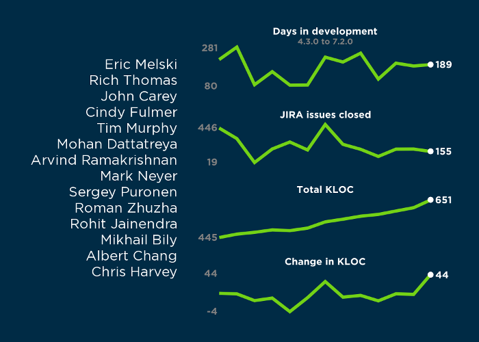
    Builds can be measured in many ways: number of output targets, number of input files, total lines of code, aggregate bytes of output generated, etc. Generally speaking, the bigger the build is, the longer it will take to complete. If your build is long simply because of its size, you may think you have no opportunities, but that’s not so: parallel builds, caching outputs, componentization and beefier hardware can all help cope with this type of problem.

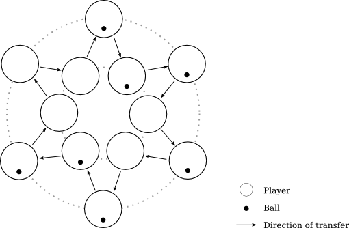
  2. Execution parallelism

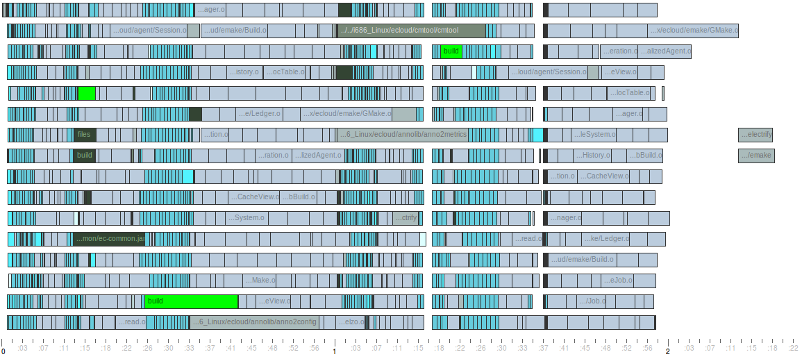
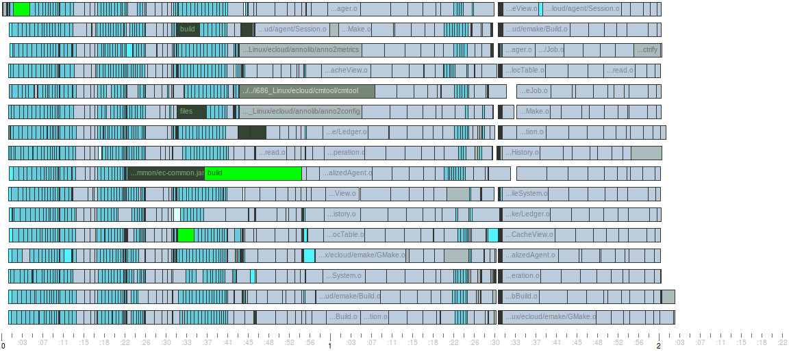
    Most build tools support some form of parallel execution — GNU make’s -j option is the classic example. Assuming there is parallelizable work in the build, the build that runs on more cores (that is, with a higher -j value) will complete more quickly.

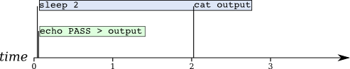
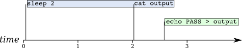
  3. Available parallelism / build structure

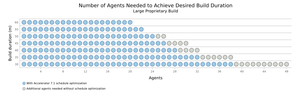
    Running a build on many cores only helps if there is exploitable parallelism in the build. If the build is defined in such a way that parallelism is limited, then it will take longer to complete regardless of the -j value. For example, some builds may have unnecessary serializations in the dependency graph, which will limit performance.

  4. Caching

    The use of (or failure to use) caching technology, such as ElectricAccelerator’s JobCache, ClearCase winkins, or ccache, can dramatically impact build performance. In my tests caching such as JobCache can reduce build duration by 50% or more for full builds.

  5. Conflicts (ElectricAccelerator only)

    For builds executed with ElectricAccelerator, conflicts can have a significant impact on performance. Briefly, an Accelerator conflict is any time your build “loses” a race condition between two steps that should have been serialized but weren’t due to missing dependencies in your makefile or build files. Accelerator can detect and correct such errors on-the-fly, but it comes at a cost. A few conflicts is usually not a problem, but if you have hundreds or thousands, it will make your build slower as Accelerator reruns portions of the build to get the correct results. Usually if you see such a scenario it’s a sign that you didn’t have a complete Accelerator history file for your build, so fixing such issues is as easy as using the history file generated by that build to augment the dependency information in future runs of the build.

  6. Code complexity and structure

    There are many attributes of the code itself which can affect build performance. For example, as a general rule, very long source files will take longer to compile than shorter files. Files containing very long individual functions will take longer to compile than files with only short functions. Heavy use of templates in C++ will cause slower compilation. Careless use of #include statements in C or C++ code will cause slower compilation and can be especially harmful to incremental builds by triggering excessive recompilation.

  7. Implementation language

    Some languages are easier to process and therefore faster to compile. In general, C++ is slower to compile, while languages like Java or Go are very quick to compile. Some languages require no compilation at all, so builds of code using such languages can be very very fast indeed!

  8. Build tool

    There are a staggering array of build tools which you might choose to drive your build: GNU make, ninja, maven, ant, scons, emake, tup and more. Some were designed for high performance on full builds, while others were designed for high performance on incremental builds, and still others were designed for ease-of-use, correctness, or other non-performance related attributes. The choice of build tool will affect the performance of your build, especially if your build is very large.

  9. Compiler

    For compiled languages like C and C++ there are often many different compilers that you could choose from for your build: gcc/g++, clang, icc, WindRiver, Microsoft cl, tcc, etc. These tools themselves have different performance profiles, and the performance may even vary from one version of the compiler to the next.

  10. Compiler options

    For a given compiler, the build options you enable may significantly affect the compile time. For example, when using gcc, building with -O3 is generally slower than building with -O0. Therefore for developer builds, you may consider to disable optimizations in order to reduce build cycle time. Other options that may influence compile speed include: pre-compiled headers (PCH); dependency generation (-MD, -MMD, -MF, etc); profiling or coverage analysis (-fprofile-arcs or -ftest-coverage); and include path definitions (-I), which if very long can cause the compiler to spend excessive time searching for header files.

  11. Linker

    As with the compiler, different linkers have different performance characteristics. For C/C++ compilation on Linux the default linker is GNU ld, but there are alternatives like Google gold which have much better performance, albeit for a subset of the use cases supported by GNU ld. If your use case is supported by gold, you will likely see much better build performance by switching.

  12. Memory

    As with any process involving computers, the amount of available memory will have a significant impact on build performance. Too little and your system will swap excessively. Fortunately there’s no such thing as “too much”, though it may be prohibitively expensive to get so much RAM that you can stop worrying about it. In practice most builds do not require a huge amount of memory, but if yours do, and you don’t have enough, your build speed will suffer.

  13. Disk performance

    Like memory, the performance of your disk can significantly affect build performance. In fact its easier in some ways to understand the impact of disk speed. If the build generates 10GB of output and your disk can only write at 10MB/s, the fastest that the build can possibly finish is about 1,000 seconds, or nearly 20 minutes. On the other hand, if the build generates only 5MB of output and uses the same disk, then only 1/2 second is needed to write the build outputs, so the disk is unlikely to be a bottleneck. You may find that the disk is adequate for your builds now, but as the build gets bigger you will reach a point where the disk is no longer fast enough. At that point you can upgrade to a faster disk, and that will be sufficient for some time until again your build grows to exceed the capacity of the disk.

    Even if your disk is not a primary bottleneck now, switching to a faster disk may improve performance somewhat. Many users have had good results from switching to SSD for temporary storage, or using striped RAID for those builds that generate truly enormous amounts of data.

  14. Network performance

    For distributed builds such as those executed with ElectricAccelerator, network performance is crucial because build data has to be transferred across the network. But even if the build itself is not distributed, it may make use of tools pulled from a network file share, so the network performance can affect the build.

  15. Operating system / kernel version

    Some operating systems have better performance for builds than others — in general, I’ve found builds on Linux to be relatively faster than builds on Windows, for example. Likewise, some versions of the operating system may be faster than others. Some users have reported as much as a 3x improvement by upgrading from an old version of Linux to a newer version due to optimizations in the kernel itself.

  16. Anti-virus software

    Use of anti-virus software can dramatically impact build performance, particularly if the A/V is configured in one of the more aggressive or intrusive modes of operation: sometimes every file operation is intercepted by the A/V scanner, adding a substantial drag on build speed.

  17. License management

    Some build tools, such as certain commercial compilers, require licenses in order to operate. If the license system is misconfigured it can add delays to the build process, sometimes causing each compile to take minutes instead of seconds as the compiler tries and fails to contact a license server, or contacts the wrong license server instance (for example, one on a different subnet).

A foundation for performance investigations

So there you have it: my (not entirely) comprehensive list of factors that can affect build performance. Of course these won’t all be relevant for every build: every build is different, and each has a unique performance profile. A slow disk may be mostly irrelevant for one build but absolutely critical for another. My hope is that this list will serve as a foundation for your build performance investigations — something to help get you started, even if it doesn’t get you all the way to a conclusion.

What do you think of my list? What would you add, and how would you change the ordering? Let me know in the comments below.

What’s new in GNU make 4.2?

In May 2016 the GNU make team released GNU make 4.2. I’m pleased to see another release, though I find myself underwhelmed by both the timeline and the content of this release. When 4.1 came out just one year after 4.0 I hoped it was a sign that the GNU make project was switching to a more frequent and regular release cycle, as many software projects have done in the last several years. Although it can be a difficult adjustment this release cadence can have significant benefits like improving user engagement and reducing risk. But with the 4.2 release arriving nineteen long months after 4.1 it seems that GNU make has failed to make the transition.

Of course infrequent releases are not necessarily a problem, as long as the releases contain compelling new functionality. Unfortunately the new features in GNU make 4.2 are charitably described as “uninspiring” — though I’m sure each enhancement will be handy for the corner case it was designed to address. Of course GNU make is a mature project by any definition, and frankly it does what it does pretty well and has for a very long time — maybe it’s just “done”. But consider this: the past few years has seen something of an explosion in the build tool space, with several new build tools cropping up. Each of the following alternative build tools has had multiple releases in the last year, and each has innovative features that could be adopted by GNU make:

  • gradle, the default build tool for Android apps. Monthly releases. Reports and notifications.
  • bazel, the open-source version of Google’s internal build system. Ten releases already in 2016. Checksum-based up-to-date checks and minimization of test suite executions.
  • ninja, a make-like build tool. Two releases in the last twelve months. Resource pools and unbelievably fast parsing / low overhead.

So, what does GNU make 4.2 have to offer? Read on to see, and let me know in the comments if you disagree with my analysis.

.SHELLSTATUS variable

GNU make has had the $(shell) function for many years. This provides a mechanism by which you can get the result (stdout) of an arbitrary command into a make variable, where you can do whatever you like with it. One curious thing about $(shell) is that it doesn’t care at all whether the command you execute succeeds or not, so if you try to read a non-existent file, for example, with $(shell cat missing.txt), GNU make will simply return an empty string as the result of the shell invocation. In some cases you may want to actually check the exit status of that command, and in GNU make 4.2 you now can, by checking the value of .SHELLSTATUS, a new built-in variable that is automatically set to the exit code of the most recent $(shell) (or != assignment). Here’s a contrived example:

1
2
3
4
5
FOO := $(shell exit 1)
ifneq ($(.SHELLSTATUS),0)
$(error shell command failed!)
endif
all: ; @echo done

As you can see, it’s now possible to make your makefile react in whatever manner you deem appropriate when a shell invocation fails. Be advised, however: if you find yourself doing this, it may be an indication that your makefile is poorly written — almost every use of $(shell) is better handled by creating an actual rule to do whatever you were going to do with $(shell).

Read files with $(file)

The $(file) function was added to GNU make in the 4.0 release, in order to enable the creation of files directly from make — quite handy for those cases in which the content you want to write is so long it exceeds command-line length limits on your system. In 4.2 the $(file) function was extended so that you can use it to read files in addition to writing files. For example, SRCS := $(file <sourcelist.txt) would capture the content of the file sourcelist.txt in the variable SRCS, less the final newline in the file, if any (that last bit is for consistency with the $(shell) function).

Improved error reporting

GNU make 4.2 includes a small but very useful improvement in error reporting: previously when make encountered an error while executing a recipe, it would report only the name of the target being built, such as make: *** [all] Error 1. Starting with 4.2, this error message includes the makefile and line number of the specific command that produced the error: make: *** [Makefile:6: all] Error 1. This should make it much easier to debug large, complex builds — especially anything that uses double-colon rules to composite functionality from many fragments in distinct makefiles.

Bug fixes

In addition to the modest enhancements described above, the 4.2 release includes about three dozen other bug fixes. A glance at the resolution dates on those reveals that sometimes months passed with no updates. This makes me wonder why they didn’t cut a release at those points, even if it were just for bug fixes. My guess is that the project is trapped, in a sense: because the interval between releases is so long there’s a sense that each release has to be “perfect”, and because there’s an attempt to ensure each release is “perfect”, the interval between releases must be very long. Contrast this with a more agile approach, which can tolerate imperfect releases because the next release is just around the corner anyway. Combined with an ever expanding automated regression test suite it’s possible to gradually increase the bar for release quality, such that in fact the likelihood of a bad release goes down when compared with a project that has a long release cycle and is dependent on mostly manual testing.

GNU make isn’t going to go away any time soon, but I think the writing is on the wall: if it doesn’t start innovating again, developers will inevitably migrate to other build tools that do.

What’s new in GNU make 4.1?

October 2014 saw the release of GNU make 4.1. Although this release doesn’t have any really remarkable new features, the release is notable because it comes just one year after the 4.0 release — that’s the least time between releases in more than a decade. Hopefully, this is the start of a new era of more frequent, smaller releases for this venerable project which is one of the oldest still active projects in the GNU suite. Read on for notes about the new features in GNU make 4.1.

MAKE_TERMOUT and MAKE_TERMERR

Starting with 4.1, GNU make defines two additional variables: MAKE_TERMOUT and MAKE_TERMERR. These are set to non-empty values if make believes stdout/stderr is attached to a terminal (rather than a file). This enables users to solve a problem introduced by the output synchronization feature that was added in GNU make 4.0: when output synchronization is enabled, all child processes in fact write to a temporary file, even though in effect they are writing to the console. In other words, the implementation details of output synchronization may interfere with behaviors in child processes like output colorization which require a terminal for correct operation. If MAKE_TERMOUT or MAKE_TERMERR is set, then the user may explicitly direct such commands to maintain colorized output despite the fact that they appear to be writing to a file.

Enhanced $(file) function

The $(file) function was added in GNU make 4.0 to enable writing to files from a makefile without having to invoke a second process to do so. For example, where previously you had to do something like $(shell echo hello > myfile), now you can instead use $(file > myfile,foo). In theory this is more efficient, since it avoids creating another process, and it enables the user to easily write large blocks of text which would exceed command-line length limitations on some platforms.

In GNU make 4.1, the $(file) function has been enhanced such that the text to be written may be omitted from the function call. This allows $(file) to work as a sort of “poor man’s” replacement for touch, although having reviewed the bug report that resulted in this change, I think this is more an “enhancement of convenience” than a deliberate attempt to evolve the program. Of course I have to give a shout out to my friend Tim Murphy, who filed the bug report that led to this enhancement — nice work, Tim!

Relaxed constraints for mixing explicit and implicit rules

The final feature change in GNU make 4.1 is that make will emit a regular error rather than a fatal error (which terminates the build) when both explicit and pattern targets are specified as outputs of a rule, like this:

1
foo bar%: baz

This is an interesting change mostly for the high level of drama surrounding it. That bit of syntax is clearly illegal — in fact, if the pattern target is listed first rather than the explicit, GNU make has long identified this as invalid syntax, terminating the parse with *** mixed implicit and normal rules. Stop. Unfortunately, due to a defect in older versions of GNU make this construct is not prohibited when the explicit rule is named first.

In 3.82, the GNU make maintainers fixed the defect: whether or not the explicit target is named first, GNU make would identify the invalid syntax and terminate parsing. Everything was fine for about a year, and then? People flipped out. As it turns out, this construct is used by a prominant open source project: the Linux kernel. The offending syntax had been eliminated from the main development branch shortly after the 3.82 release, but third-party developers suddenly found themselves unable to build legacy versions of the kernel with the latest release of GNU make. A bug report was filed and generated 21 reponses, when the average GNU make bug report has only 3. Ultimately, the maintainers relented by reducing the severity to a non-fatal error for the 4.1 release — but with a stern message that this will likely become a fatal error again in a future release.

Bug fixes and thoughts

In addition to the bigger items identified above, the 4.1 release includes about two dozen other bug fixes. Overall, this release feels like a minor one — as often happens when release frequency increases, the individual releases become less interesting. From an agile/continuous delivery standpoint, that’s exactly what you want. But I’ve found that it is also difficult for a team that’s accustomed to less frequent releases with larger payloads to transition to smaller, more frequent releases while still incorporating large changes that take longer than one release to implement. Of course, one point does not make a line — that is, we can’t tell from this release alone whether the intention is to switch to a more frequent release cadence, or whether this release is an exception. If they are trying to increase the frequency, I think it will be very interesting to see how the GNU make development team adapts to the new cadence. Regardless, I’d like to congratulate the team for this release and I look forward to seeing what comes next.

HOWTO: Intro to GNU make variables

One thing that many GNU make users struggle with is predicting the value of a variable. And it’s no wonder, with the way make syntax freely mingles text intended for two very distinct phases of execution, and with two “flavors” of variables with very different semantics — except, that is, when the one seems to behave like the other. In this article I’ll run you through the fundamentals of GNU make variables so you can impress your friends (well, your nerdy friends, anyway) with your ability to predict the value of a GNU make variable at social gatherings.

Contents

Basics

Let’s start with the basics: a GNU make variable is simply a shorthand reference for another string of text. Using variables enables you to create more flexible makefiles that are also easier to read and modify. To create a variable, just assign a value to a name:

1
CFLAGS=-g -O2

Later, when GNU make sees a reference to the variable, it will replace the reference with the value of the variable — this is called expanding the variable. A variable reference is just the variable name wrapped in parenthesis or curly braces and prefixed with a dollar-sign. For example, this simple makefile will print “Hello, world!” by first assigning that text to a variable, then dereferencing the variable and using echo to print the variable’s value:

1
2
3
MSG = Hello, world!
all:
@echo $(MSG)

Creating variables

NAME = value is just one of many ways to create a variable. In fact there are at least eight ways to create a variable using GNU make syntax, plus there are built-in variables, command-line declarations, and of course environment variables. Here’s a rundown of the ways to create a GNU make variable:

  • MYVAR = abc creates the variable MYVAR if it does not exist, or changes its value if it does. Either way, after this statement is processed, the value of MYVAR will be abc.
  • MYVAR ?= def will create the variable MYVAR with the value def only if MYVAR does not already exist.
  • MYVAR += ghi will create the variable MYVAR with the value if MYVAR does not already exist, or it will append ghi to MYVAR if it does already exist.
  • MYVAR := jkl creates MYVAR if it does not exist, or changes its value if it does. This variation is just like the first, except that it creates a so-called simple variable, instead of a recursive variable — more on that in a minute.

In addition to the various assignment operators, you can create and modify variables using the define directive — handy if you want to create a variable with a multi-line value. Besides that, the define directive is equivalent to the normal VAR=VALUE assignment.

1
2
3
4
define MYVAR
abc
def
endef

If you’re using GNU make 3.82 or later, you can add assignment operators to the define directive to modify the intent. For example, to append a multi-line value to an existing variable:

1
2
3
4
define MYVAR +=
abc
def
endef

But there are still more ways to create variables in GNU make:

  • Environment variables are automatically created as GNU make variables when GNU is invoked.
  • Command-line definitions enable you to create variables at the time you invoke GNU make, like this: gmake MYVAR=123.
  • Built-in variables are automatically created when GNU make starts. For example, GNU make defines a variable named CC which contains the name of the default C compiler (cc) and another named CXX which contains the name of the default C++ compiler (g++).

Variable flavors

Now that you know how to create a GNU make variable and how to dereference one, consider what happens when you reference a variable while creating a second variable. Let’s use a few simple exercises to set the stage. For each, the answer is hidden on the line following the makefile. You can reveal the answer by highlighting the hidden text in your browser.

  1. Q1: What will this makefile print?
    1
    2
    3
    4
    ABC = Hello!
    MYVAR = $(ABC)
    all:
    @echo $(MYVAR)

    A1: Hello!

  2. Q2: What will this makefile print?
    1
    2
    3
    4
    5
    6
    ABC = Hello!
    MYVAR = $(ABC)
    all:
    @echo $(MYVAR)
    ABC = Goodbye!

    A2: Goodbye!

  3. Q3: What will this makefile print?
    1
    2
    3
    4
    5
    6
    ABC = Hello!
    MYVAR := $(ABC)
    all:
    @echo $(MYVAR)
    ABC = Goodbye!

    A3: Hello!

Don’t feel bad if you were surprised by some of the answers! This is one of the trickiest aspects of GNU make variables. To really understand the results, you have to wrap your brain around two core GNU make concepts. The first is that there are actually two different flavors of variables in GNU make: recursive, and simple. The difference between the two is in how GNU make handles variable references on the right-hand side of the variable assignment — for brevity I’ll call these “subordinate variables”:

  • With simple variables, subordinate variables are expanded immediately when the assignment is processed. References to subordinate variables are replaced with the value of the subordinate variable at the moment of the assignment. Simple variables are created when you use := in the assignment.
  • With recursive variables, expansion of subordinate variables is deferred until the variable named on the left-hand side of the assignment is itself referenced. That leads to some funny behaviors, because the value of the subordinate variables at the time of the assignment is irrelevant — in fact, the subordinate variables may not even exist at that point! What matters is the value of the subordinate variables when the LHS variable is expanded. Recursive variables are the default flavor, and they’re created when you use simply = in the assignment.

The second concept is that GNU make processes a makefile in two separate phases, and each phase processes only part of the text of the makefile. The first phase is parsing, during which GNU make interprets all of the text of the makefile that is outside of rule bodies. During parsing, rule bodies are not interpreted — only extracted for processing during the second phase: execution, or when GNU make actually starts running the commands to update targets. For purposes of this discussion, that means that the text in rule bodies is not expanded until after all the other text in the makefile has been processed, including variable assignments that physically appear after the rule bodies. In the following makefile, the text highlighted in green is processed during parsing; the text highlighted in blue is processed later, during execution. Again, to put a fine point on it: all of the green text is processed before any of the blue text:

1
2
3
4
5
6
ABC = Hello!
MYVAR = $(ABC)
all:
@echo $(MYVAR)
ABC = Goodbye!

Now the examples above should make sense. In Question 2, we created MYVAR as a recursive variable, which means the value of ABC at the time MYVAR is created doesn’t matter. By the time GNU make needs to expand MYVAR, the value of ABC has changed, so that’s what we see in the output.

In Question 3, we created MYVAR as a simple variable, so the value of ABC was captured immediately. Even though the value of ABC changes later, that change doesn’t affect the value of MYVAR.

Target-specific variables

Most variables in GNU make are global: that is, they are shared across all targets in the makefile and expanded the same way for all targets, subject to the rules outlined above. But GNU make also supports target-specific variables: variables given distinct values that are only used when expanding the recipe for a specific target (or its prerequisites).

Syntactically, target-specific variables look like a mashup of normal variable definitions, using =, :=, etc.; and prerequisite declarations. For example, foo: ABC = 123 creates a target-specific definition of ABC for the target foo. Even if ABC has already been defined as a global variable with a different value, this target-specific definition will take precedence when expanding the recipe for foo. Consider this simple makefile:

1
2
3
4
5
6
7
8
ABC = Hello!
all: foo bar
foo:
@echo $(ABC)
bar: ABC = Goodbye!
bar:
@echo $(ABC)

At first glance you might expect this makefile to print “Goodbye!” twice — after all, ABC is redefined with the value “Goodbye!” before the commands for foo are expanded. But because the redefinition is target-specific, it only applies to bar. Thus, this makefile will print one “Hello!” and one “Goodbye!”.

As noted, target-specific variables are inherited from a target to its prereqs — for example, the following makefile will print “Surprise!”, because bar inherits the target-specific value for ABC from foo:

1
2
3
4
5
6
ABC = Normal.
foo: ABC = Surprise!
foo: bar
bar:
@echo $(ABC)

You can do some neat tricks with this, but I urge you not to rely on the behavior, because it doesn’t always work the way you might think. In particular, if a target is listed as a prereq for multiple other targets, each of which have a different target-specific value for some variable, the actual value used for the prereq may vary depending on which files were out-of-date and the execution order of the targets. As a quick example, compare the output of the previous makefile when invoked with gmake foo and when invoked with gmake bar. In the latter case, the target-specific value from foo is never applied, because foo itself was not processed. With GNU make 3.82 or later, you can prevent this inheritence by using the private modifier, as in foo: private ABC = Surprise!.

Finally, note that target-specific variables may be applied to patterns. For example, a line reading %.o: ABC=123 creates a target-specific variable for all targets matching the pattern %.o.

Conclusion

If you’ve made it this far, you now know just about everything there is to know about GNU make variables. Congratulations! I hope this information will serve you well.

Questions or comments? Use the form below or hit me up on Twitter @emelski.

The ElectricAccelerator 7.2 “Ship It!” Award

Naturally with the release of ElectricAccelerator 7.2 a few weeks ago it’s time for another Accelerator “Ship It!” award. In keeping with our tradition, I gave each team member a LEGO figure that symbolized the release to me in some way, along with a a custom trading card giving the vital details: version, release date, and key features. Like a baseball card, the back is filled with a team roster and release statistics.

There are some great improvements in Accelerator 7.2 but there’s no particular unifying theme, so it was quite a challenge to choose a suitable minifig. One thing that stood out is that between the time management asked engineering to create a 7.2 release and the time that development was complete was only about three weeks. At the time we were actually in the midst of development on another release entirely, with a different set of new features. The 7.2 release was very much a, “Hey couldn’t you also cut a release right now while you’re at it?” And we did. Maybe it’s not as impressive as those guys that can cut a release every minute of every day, but for a team that usually does releases on a six-month cadence, a 3-week turnaround sounds like continuous delivery to me.

One thing enabled us to turn around the release that quickly: our code is (nearly) always shippable. That’s what led me to the minifig for this release: the sea captain, who’s always ready to “ship out” on short notice. Here’s the trading card that accompanied the figure:

Accelerator 7.2 "Ship It!" Card Front - click for larger version

Accelerator 7.2 “Ship It!” Card Front – click for full-size version

Accelerator 7.2 "Ship It!" Card Back - click for larger version

Accelerator 7.2 “Ship It!” Card Back – click for full-size version

Like the 7.1 card, the back of the 7.2 card incorporates stats for the current release, contextualized by stats for several previous releases:

  • Number of days in development. This is just the number of days since the previous feature release — it is assumed that whatever features are in the new release, we started working on them more-or-less after the last release went out.
  • JIRA issues closed.
  • Total KLOC. This metric gives the total size of the Accelerator code base in thousands of lines of code, as measured with the excellent Count Lines of Code utility by Al Danial. This measurement excludes comments and whitespace.
  • Change in KLOC. This is simply the arithmetic difference between the total KLOC for each release and its predecessor.

As always, my sincere gratitude goes to everybody on the Accelerator team, without whom this release would not have been. Thank you!

What’s new in ElectricAccelerator 7.1

ElectricAccelerator 7.1 hit the streets a last month, on October 10, just six months after the 7.0 release in April. There are some really cool new features in this release, which picks up right where 7.0 left off by adding even more ground-breaking performance features: schedule optimization and Javadoc caching. Here’s a quick look at each.

Schedule Optimization

The idea behind schedule optimization is really simple: we can reduce overall build duration if we’re smarter about the order in which jobs are run. In essense, it’s about packing the jobs in tighter, eliminating idle time in the middle of the build and reducing the “ragged right edge”. Here’s a side-by-side comparison of the same build, first using normal scheduling and then using schedule optimization. You can easily see that schedule optimization made the second build faster — an 11% improvement in this small, real-world example:

Build using naive scheduling -- click to view full size

Build using naive scheduling — click to view full size

Build using schedule optimization - click to view full size

Build using schedule optimization – click to view full size

If you study the two runs more closely, you can see how schedule optimization produced this improvement: key jobs, in particular the longest jobs, were started earlier. As a result, idle time in the middle of the build was reduced or eliminated entirely, and the right edge is much less uneven. But the best part? It’s completely automatic: all you have to do is run the build once for emake to learn its performance profile. Every subsequent build will leverage that data to improve build performance, almost like magic.

Not convinced? Here’s a look at the impact of schedule optimization on another, much bigger proprietary build (serial build time 18h25m). The build is already highly parallelizable and achieves an impressive 37.2x speedup with 48 agents — but schedule optimization can reduce the build duration by nearly 25% more, bringing to total speedup on 48 agents to an eye-popping 47.5x!

Build duration with naive and optimized scheduling

Build duration with naive and optimized scheduling

There’s another interesting angle to schedule optimization though. Most people will take the performance gains and use them to get a faster build on the same hardware. But you could go the other direction just as easily — keep the same build duration, but do it with dramatically less hardware. The following graph quantifies the savings, in terms of cores needed to achieve a particular build duration. Suppose we set a target build duration of 30 minutes. With naive scheduling, we’d need 48 agents to meet that target. With schedule optimization, we need only 38.

Resource requirements with naive and optimized scheduling - click for full size

Resource requirements with naive and optimized scheduling – click for full size

I’m really excited about schedule optimization, because it’s one of those rare features that give you something for nothing. It’s also been a long time coming — the idea was originally conceived of over three years ago, and it’s only now that we were able to bring it to fruition.

Schedule optimization works with emake on all supported platforms, with all emulation modes. It is not currently available for use with electrify.

Javadoc caching

The second major feature in Accelerator 7.1 is Javadoc caching. Again, it’s a simple idea: think “ccache”, but for Javadoc instead of compiles. This is the next phase in the evolution of Accelerator’s output reuse initiative, which began in the 7.0 release with parse avoidance. Like any output reuse feature, Javadoc caching works by capturing the product of a Javadoc invocation and storing it in a cache indexed by a hash of the inputs used — including the Java files themselves, the environment variables, and the command-line. In subsequent builds, emake will check those inputs again and if it computes the same hash, emake will used the cached results instead of running Javadoc again. On big Javadoc jobs, this can produce significant savings. For example, in the Android “Jelly Bean” open-source build, the main Javadoc invocation usually takes about five minutes. With Javadoc caching in Accelerator 7.1, that job runs in only about one minute — an 80% reduction! In turn that gives us a full one minute reduction in the overall build time, dropping the build from 13 minutes to 12 — nearly a 10% improvement:

Uncached Javadoc job in Android build - click for full image

Uncached Javadoc job in Android build – click for full image

Cached Javadoc job in Android build - click for full build

Cached Javadoc job in Android build – click for full image

Javadoc caching is available on Solaris and Linux only in Accelerator 7.1.

Looking ahead

I hope you’re as excited about Accelerator 7.1 as I am — for the second time this year, we’re bringing revolutionary new performance features to the table. But of course our work is never done. We’ve been hard at work on the “buddy cluster” concept for the next release of Accelerator. Hopefully I’ll be able to share some screenshots of that here before the end of the year. We’re also exploring acceleration for Bitbake builds like the Yocto Project. And last, but certainly not least, we’ll soon start fleshing out the next phase of output reuse in Accelerator — caching compiler invocations. Stay tuned!

The inverted parallel build bug

At some point most of you have encountered “the” parallel build problem: a build that works just fine when run serially, but breaks sometimes when run in parallel. You may have read my blog about how ElectricAccelerator automatically solves the classic parallel build problem. Recently I ran into the opposite problem in a customer’s build: a build that “works” when run in parallel, but breaks when run serially! If you’re lucky, this build defect will just cause occasional build failures. If you’re unlucky, it will silently corrupt your build output at random. With traditional GNU make this nasty bug is a nightmare to track down — if you even know that its present!

In contrast, the unique features in ElectricAccelerator make it trivial to find the defect — some might even say it’s fun (well, if you’re like me and you enjoy using powerful tools to do sophisticated analysis without breaking a sweat!). Read on to see how ElectricAccelerator makes it easy to diagnose and fix bugs in your build.

The inverted parallel build bug

Let’s start with a concrete example. Here’s a simple Makefile which (appears to) work when run in parallel, but which consistently fails serially:

1
2
3
4
5
6
7
8
all: reader writer
reader:
sleep 2
cat output
writer:
echo PASS > output

Assuming that output does not exist, executing this makefile serially will always produce an error:

$ gmake
sleep 2
cat output
cat: output: No such file or directory
gmake: *** [reader] Error 1

But if you execute this makefile in parallel, it appears to work!:

$ gmake -j 2
sleep 2
echo PASS > output
cat output
PASS

If we visualize the execution of these commands it’s easy to see why the parallel build seems to work:

Sample parallel execution timeline

At the beginning of the build, both reader and writer are started, more-or-less at the same time, because we told gmake to run two jobs at a time. reader has two commands, which are executed serially according to the semantics of make. While the sleep 2 is executing, the echo command in writer runs and completes. When the cat command in reader starts, it succeeds because output is ready-to-go.

Parallel execution is no guarantee

Some people will look at that explanation and think “Got it — always run this thing in parallel and we’re good!” Of course, you can’t really be 100% sure that everybody will remember to run the makefile in parallel. But even if you could, there’s a flaw in that reasoning: basically, your build has a race condition, and there’s no guarantee that you’ll “win” the race every time. For example, if your build server is heavily loaded, the sequence of events might look like this instead:

Alternative parallel execution timeline

Here, writer doesn’t get started until after the sleep command has finished — too late to save the cat command from failure.

Build failure is not the worst outcome

Before we move on to finding and fixing problems like this, let’s take a quick look at one more failure mode: incremental builds. In particular, check out what happens if output exists before the build starts, but with incorrect content (for example, stale data from an earlier build):

$ echo '*** FAIL ***' > output
$ gmake
sleep 2
cat output
*** FAIL ***
echo PASS > output
$ echo $?
0

That’s right — the build “succeeded”, because it produced no error messages and exited with a zero exit code. And yet, it produced completely bogus output. Ouch!

Somebody save me!

If you’re using ordinary GNU make, you’re in for a world of hurt with a problem like this. First, the only way to consistently reproduce the problem is to run the entire build serially — of course that probably takes a long time, or you wouldn’t have been using parallel builds in the first place. Second, there are no diagnostics built into gmake that could help you identify which job produces output. One option is to use strace to monitor filesystem accesses, but that will generate a mountain of data in a not-very-usable format. Plus, it imposes a substantial performance penalty — on top of the hit you’d already take for running the build serially. Yuck!

If you’re using Electric Make, this problem is embarrassingly easy to solve thanks to emake’s core features:

  • Consistent results: emake mimics serial execution with gmake, so you’ll always get a consistent result with this build. That means it will fail, the same way, every time, which means you’ll discover the problem immediately after it is introduced, not months or years later after it has become nearly impossible to tell which Makefile change introduced the defect.
  • Parallel speed: emake’s results match those of a serial gmake build, but its performance is more like that of a parallel gmake build — better, in most cases.
  • Annotated build logs: emake can generate an XML-enhanced version of the build output log which contains a record of every file accessed by every job in the build. This annotation file can easily be mined to identify pairs of jobs where the reader preceeds the writer.

You can use any general purpose XML parsing library to read annotation files, but it’s easy to use annolib, the high-performance annotation processing library we wrote to facilitate this kind of analysis. Since annolib is built into ElectricInsight, the easiest way to use it is to write the analysis as a custom Insight report. All you need to do is iterate through the files referenced in the build, looking for read operations (or, in this case, failed lookups) preceeding a write operation. Here’s the code:

global anno
set instances [list]

# Iterate over the files referenced in the build...

foreach filename [$anno files] {
    set readers [list]

    # Iterate over the operations performed on the file...

    foreach tuple [$anno file operations $filename] {
        foreach {job op dummy} $tuple { break }
        if { $op == "read" || $op == "failedlookup" } {
            # If this is a read operation, note the job that did the read.

            lappend readers $job
        } elseif {$op == "create" || $op == "modify" || $op == "truncate"} {
            # If this is a write operation but earlier jobs already read
            # the file, we've found a read-before-write instance.

            if { [llength $readers] } {
                lappend instances [list $readers $job $filename]
            }

            # After we see a write on this file we can move on to the next.

            break
        }
    }
}

# For each instance, print the filename, the writer, and each reader.

set result ""
foreach instance $instances {
    foreach {readers writer filename} $instance { break }
    set writerName [$anno job name $writer]
    set writerFile [$anno job makefile $writer]
    set writerLine [$anno job line $writer]
    append result "FILENAME:\n  $filename\n"
    append result "WRITER  :\n  $writerName ($writerFile:$writerLine)\n"
    append result "READERS :\n"
    foreach reader $readers {
        set readerName [$anno job name $reader]
        set readerFile [$anno job makefile $reader]
        set readerLine [$anno job line $reader]
        append result "  $readerName ($readerFile:$readerLine)\n"
    }
}

With a bit of additional boilerplate you can run this report from the command-line with Insight 4.0 (currently in limited beta). A couple notes on usage: you should instruct emake to generate lookup-level annotation, by adding –emake-annodetail=lookup to your invocation. And, you should run the build with the -k (keep-going) option — otherwise, the error in reader will prevent writer from running, and emake will not record filesystem usage for it. Once you have a suitable annotation file, here’s how the report looks for this build:

$ einsight --report=ReadBeforeWrite emake.xml
done.
FILENAME:
/home/ericm/test/output
WRITER :
writer (Makefile:7)
READERS :
reader (Makefile:3)

Voila! We’ve pinpointed the problem with barely 50 lines of code (including comments!). You can even see a solution: add writer as a prerequisite of reader, on line 3 of Makefile.

Show me what you can do with ElectricAccelerator

As you’ve seen, ElectricAccelerator makes it easy to identify and correct build problems that would otherwise be nearly impossible to root out. Hopefully you also see that this is just the tip of the iceberg — with consistent fast builds and the treasure trove of data available in annotation files, what other analysis could you do? To get started, you can download a free trial of ElectricAccelerator Developer Edition and check out the reports in ElectricInsight. You can also download the Read Before Write report for ElectricInsight from my GitHub repo. If you come up with something cool, tell me about it in the comments!

try_eade_button2

The ElectricAccelerator 7.0 “Ship It!” Award

With ElectricAccelerator 7.0 out the door, it’s finally time for the moment you’ve all been waiting for: the unveiling of the Accelerator 7.0 “Ship It!” award. This time I picked the Clockwork Android, in light of our emphasis on Android build performance. Here’s the trading card that accompanied the figure:

BEEP BOP BOOP

BEEP BOP BOOP

metrics metrics metrics metrics

metrics metrics metrics metrics

As with the 6.2 award, I included some metrics about the release:

  • Number of days in development. This release was relatively long compared to our other releases — not quite our longest development cycle, but close. That’s partly because this release encompassed the Thanksgiving and Christmas seasons, which typically costs us 3-4 weeks of development and testing time. We also deliberately pushed out the release date about 2 weeks to incorporate feedback from beta testers.
  • JIRA issues closed. We resolved 185 issues in this release. That’s double what we had in 6.2, and it includes some really cool new features.
  • Performance improvement. Since this release was all about performance, it made sense to include the data that proves our success. I had some trouble finding a good way to visualize the improvement, but I’m happy with the finished product.

Of course, none of the achievements in Accelerator 7.0 would have been possible without the hard work and dedication of the incredibly talented Accelerator team. Thank you all!

“Playing” with agile

Recently we invited a Scrum coach to Electric Cloud to teach us how to get started with the Scrum model of agile development. On the first day we played a game intended to introduce us to the core elements of Scrum: plan, do, inspect, adapt (or “plan, do, check, act”; or “the Deming cycle”). Without getting into a deeper discussion of Scrum itself, I thought I would share my team’s performance in this fun little game. If you’re familiar with ElectricAccelerator, our game strategy will come as no surprise: it exploits parallel processing and horizontal scalability to improve performance.

The game was simple: we were given a bucket of rubber bouncy balls and instructed to pass balls from person to person, until every member of the team had touched the ball. For each ball that completed the circuit we earned one point; for each drop we were penalized three points. A few rules made the game more interesting. First, it was forbidden for two people to touch a ball at the same time — there had to be “air time” between individuals. Second, we could not pass balls to the person directly to our left or to our right. Finally, there was a time limit (just like a sprint): we had only 2 minutes to pass balls in each round.

At the start of the game, we were given 5 minutes to plan our strategy and make a prediction of how many balls we would pass. Between each round we had 3 minutes more to modify our strategy based on our experience in the previous round and make a new prediction for the next round. If you are familiar with Scrum you’ll recognize the analogy to story points.

In total we had 12 players plus one scribe (me) that was tasked with counting the number of balls passed and dropped.

Round 1 (plan: 0; actual: 29)

Our first planning phase was best described as chaotic. It wasn’t actually clear who was on our team or not, due to some stragglers to the activity. We weren’t sure about the constraints. Everybody had ideas about how best to pass the balls, so everybody was talking at once. It seemed simple, but in fact we had barely gotten everybody in place when the 5 minute prep time elapsed. We did manage to agree on the three key elements of our strategy though:

  • Dropping balls into the cupped hands of the receiver, rather than throwing them, to minimize the risk of dropping balls.
  • Two rings of players, one inner and one outer, facing each other. Balls would be passed in a zig-zag between the rings.
  • Parallel passing. Everybody would be either passing or receiving at all times.

This diagram shows the positions of the players, as well as which players had a ball at the start of the round:

Scrum game, round 1

As you can see, we had too many balls “in play” when we started, given our strategy — a direct consequence of unclear communication during the planning phase. The surplus balls were dropped almost immediately. Our final score for this round was 29: 1 point for each of 35 balls passed, minus 6 points for 2 balls dropped.

Round 2 (plan: 50; actual: 72)

Round 1 demonstrated that our core strategy was sound, but to improve performance we decided to make a couple tweaks. First, we made certain that we were in agreement about which players would start with balls: only those in the outside ring. Second, we realized we could improve throughput by passing two balls at a time, instead of just one. With our drop-into-cupped-hands strategy this was hardly more risky than one ball at a time. We predicted that we would pass 50 balls, about 60% more than we did in round 1. Here’s the updated diagram showing the starting positions of the players and balls for round 2:

Scrum game, round 2

Our score in round 2 was 72: 72 balls passed, with zero dropped.

Round 3 (plan: 120; actual: 60)

At this point we believed we had everything worked out. We increased the balls-per-pass to three and predicted that this would result in about 120 balls passed. But during the planning phase one of our players abruptly left — to be honest I’m not even sure who it was or why they stepped away. All I know is that suddenly we had only 11 players instead of 12, which left us with 6 on the outer ring but only 5 on the inner ring. We didn’t realize the problem until people started lining up in position near the end of the planning period. With the clock ticking we made an exceptionally poor decision about how to handle the mismatch: one of the inner ring players would serve as receiver for two of the outer ring players. First they would receive from player A, then pass to player B; then immediately receive the balls back from player B before sending them on to player C. Sounds complicated, right? It was. Here’s the updated diagram:

Scrum game, round 3

This proved was disastrous for our performance. At speed, it was (understandably) hard for the player serving double-duty to efficiently execute the elaborate sequence of exchanges. In addition, we were careless when we grabbed the extra balls we needed: although most were consistently round, a few were those oddly shaped rubber rocks which move in unpredictable ways. These misshapen lumps of rubber are just a bit harder to catch than regular balls, and that slowed us down. Our final score in this round was just 57: 60 balls passed, one dropped.

Round 4 (plan: 120; actual: 123)

The obvious problem in round three was the mismatch in the sizes of the inner and outer rings. The solution was obvious too: remove one player from the outer ring to restore equilibrium. There was just one problem. According to the rules of the game, a ball had to be touched by every player in order to count as having been passed. What could we do? We pled our case to the coach, who agreed to let us have one person sit out this round — a demonstration of another fact of agile development: sometimes a team can be made more productive by having fewer people on it. With 5 players on each ring, we again predicted that we would pass 120 balls. Here’s how the layout looked for this round:

Scrum game, round 4

This was our best round yet with a final score of 123: 135 balls passed, with only four drops.

Review

Overall I was really pleased with our performance in this game — granted, the point of the exercise was not actually to see how many balls we could pass around, but to experience the plan-do-inspect-adapt cycle directly. And we certainly did that too. But come on! How can you not be excited by a more than 4x improvement in throughput from round 1 to round 4? I’m not surprised though. After all, speed is the name of the game for ElectricAccelerator. This is what we do. That we got there by applying the same strategies to this game that we use in Accelerator itself — icing on the cake.

Later that night I realized an error in our execution on round 4 though. We chose to even out the rings by dropping one player from the outer ring, when we could just as easily have added a player to the inner ring: me. As scribe, I did not actively participate in the ball passing, only the planning and review. But there was no particular reason I couldn’t have stepped in. That would have increased our throughput by 20% (by increasing the number of balls in play from 15 to 18). I think we could have exceeded 150 balls passed with that configuration. So in the end, the game was a great demonstration of what is probably the most important concept from Scrum: there’s always room for improvement.

What is the fastest way to find non-zero bits in an MD5 hash?

Microbenchmarks, as a general rule, are a waste of time. Let’s just get that out of the way up front. They are also, as a general rule, totally inaccurate, measuring the execution time of some snippet of code in a context that is completely divorced from the reality in which that code will actually be used. So if after reading this article you think, “I should tell Eric what a waste of time this was!” — don’t bother. I already know.

But… microbenchmarks are also fun, and sometimes interesting, and often vastly easier to implement than a real benchmark of the same code in a production system. So a couple weeks ago, when my colleague proposed using an MD5 hash with value zero as a sentinal indicating that the checksum had not yet been calculated, I wondered: what is the fastest way to test if an MD5 hash has any non-zero bits? I had some time to kill so I wrote a microbenchmark comparing several implementations. The results are presented here for your amusement and edification.

The benchmark

The goal of the benchmark is to determine which of several methods can most quickly determine whether an MD5 hash is all zeroes. An MD5 hash is 128 bits long, so in essence this problem boils down to simply checking for non-zero bits in an arbitrary sequence of 16 bytes. You can find the benchmark source code in my Github repo.

For sample data I simply allocated about 100,000 17 byte arrays, then set one byte in each to a non-zero value. This structure made it wasy to easily test the effect of memory alignment on performance, by using either the first 16 or the last 16 bytes of each 17 byte array as the value under test. The total size was significant as well: smaller than the L1 cache on a typical modern CPU, so we avoid measuring memory bandwidth performance.

I tested the following methods for determining whether a hash is all zero, in both aligned and unaligned varieties:

  1. Naive loop over bytes: the most obvious approach simply loops over the bytes, testing each in turn.
  2. Unrolled loop over bytes: loop unrolling is a common optimization for loops with a fixed number of iterations.
  3. Bitwise OR of bytes: OR all bytes together, then compare the result to zero.
  4. Slice by four: treat the 16 bytes as an array of four 32-bit integers, testing each for equality with zero.
  5. Slice by eight: treat the 16 bytes as an array of two 64-bit integers, testing each for equality with zero.
  6. Find first set: use the GCC builtin function __builtin_ffs, which finds the first non-zero bit in a 32-bit integer.

The code was compiled to 64-bit binaries using GCC 4.7.2 with -O2 optimization and no debugging symbols.

The results

I ran the benchmarks on two systems. First I tried a quad-core hyperthreaded 1.73GHz Intel Core i7 laptop with 16GB RAM and an SSD hard drive. All cores were put into performance mode to ensure no CPU frequency scaling was enabled, using (for example) echo performance | sudo tee /sys/devices/system/cpu/cpu0/cpufreq/scaling_governor. Here are the results (longer is better):

Comparison of strategies for finding zero-valued MD5 hashes (Intel)

The results are a bit erratic, to be sure — for example, it makes no sense that the unaligned version of the unrolled naive loop should be faster than the aligned version. This is likely just because the operation being measured is so fast that it’s hard to get a “pure” measurement: even tiny fluctuations in system load perturb the tests. You’ll see that if you run the benchmark a few times, you’ll get slightly different results each time. That just means that we shouldn’t make any hard-and-fast decisions based on the exact numbers here.

Nevertheless, the difference between slice-by-four or slice-by-eight and the other strategies is substantial enough that I trust the overall result, if not the exact numbers. That is, slice-by-four and slice-by-eight are clearly significantly faster than any other approach. But — and here’s where we discover the degree of yak shaving we’ve been up to — even the slowest strategy is still pretty damn fast. In all honesty, it is not going to make a lick of difference in overall application performance, unless you really do need to do billions of these checks. A realistic upper bound for my application is maybe ten million, which would consume a tiny fraction of a second using even the naive loop.

One final surprise in this data is the difference in performance between aligned and unaligned memory access — or rather, the lack therof. Conventional wisdom is that you pay a performance penalty for accessing unaligned memory, at least when you try to treat it as 32- or 64-bit blocks. In fact, this result supports other tests which indicate that on the Intel Core i7 there is effectively no penalty for unaligned memory access.

If you’re only working on x86 architectures, you may consider this exercise concluded. But we actually run our software on SPARC architecture as well, so before committing to an implementation let’s take a look at how the benchmark behaves there. This time I used a 1GHz SPARCv9 CPU:

Comparison of strategies for finding zero-valued MD5 hashes (SPARC)

Slice-by-four and slice-by-eight are fastest here too, as long as the data is aligned. If not — BOOM! The application crashes with a bus error, because the SPARC architecture is actually quite sensitive to data alignment. If you want to treat a piece of memory as an integer, it had better be properly aligned.

Conclusion

Informed by these results, we opted to use the slice-by-four strategy. That required a modification of our code, which previously did not guarantee alignment of MD5 hashes. Fortunately that modification was trivial, so it cost us little time and did not make the code any less clear. But you can see hints of the real danger of microbenchmarks: it’s often difficult for a developer to ignore the existence of a faster-but-more-complex strategy, despite evidence that the simple implementation is more than adequately performant. In this case the cost of enabling the faster implementation was negligable, but I’ve seen developers (including myself) needlessly contort code in the name of performance, doggedly defending their choices with microbenchmarks like these. Don’t let yourself become another statistic: use microbenchmarks, sure, but always evaluate the results in the larger context of overall application performance.

With that, I invite you to sound off in the comments: what did I overlook in my microbenchmark? How were the tests flawed? What other strategies do you know for testing whether a series of 16 bytes contains any non-zero bits?