What’s new in ElectricAccelerator 7.0

ElectricAccelerator 7.0 was officially released a couple weeks ago now, on April 12, 2013. This version, our 26th feature release in 11 years, incorporates performance features that are truly nothing less than revolutionary: dependency optimization and parse avoidance. To my knowledge, no other build tool in the world has comparable functionality, is working on comparable functionality or is even capable of adding such functionality. Together these features have enabled us to dramatically cut Android 4.1.1 (Jelly Bean) build times, compared to Accelerator 6.2:

  • Full, from-scratch builds are 35% faster
  • “No touch” incremental builds are an astonishing 89% faster

In fact, even on this highly optimized, parallel-friendly build, Accelerator 7.0 is faster than GNU make, on the same number of cores. On a 48-core system gmake -j 48 builds Android 4.1.1 in 15 minutes. Accelerator 7.0 on the same system? 12 minutes, 21 seconds: 17.5% faster.

Read on for more information about the key new features in ElectricAccelerator 7.0.

Dependency optimization: use only what you need

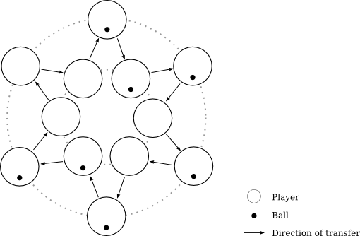
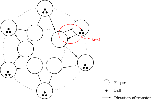
Dependency optimization is a new application of the data that is used to power Accelerator’s conflict detection and correction features. But where conflict detection is all about finding missing dependencies in makefiles, dependency optimization is focused on finding surplus dependencies, which drag down build performance by needlessly limiting parallelism. Here’s a simple example:

1
2
3
4
5
foo: bar
@echo abc > foo && sleep 10
bar:
@echo def > bar && sleep 10

In this makefile you can easily see that the dependency between foo and bar is superfluous. Unfortunately GNU make is shackled by the dependencies specified in the makefile and is thus obliged to run the two jobs serially. In contrast, with dependency optimization enabled emake can detect this inefficiency and ignore the unnecessary dependency — so foo and bar will run in parallel.

Obviously you could trivially fix this simple makefile, but in real-world builds that may be difficult or impossible to do manually. For example, in the Android 4.1.1 build, there are about 2 million explicitly specified dependencies in the makefiles. For a typical variant build, only about 300 thousand are really required: over 85% of the dependencies are unnecessary. And that's in the Android build, which is regarded by some as a paragon of parallel-build cleanliness — imagine the opportunities for improvement in builds that don't have Google's resources to devote to the problem.

To enable dependency optimization in your builds, add --emake-optimize-deps=1 to your emake command-line. The first build with that option enabled will "learn" the characteristics of the build; the second and subsequent builds will use that information to improve performance.

Parse avoidance: the fastest job is the one you don't have to do

A common complaint with large build systems is incremental build performance — specifically, the long lag between the time that the user invokes make and the time that make starts the first compile. Some have even gone so far as to invent entirely new build tools with a specific focus on this problem. Parse avoidance delivers similar performance gains without requiring the painful (perhaps impossible!) conversion to a new build tool. For example, a "no touch" incremental build of Android 4.1.1 takes close to 5 minutes with Accelerator 6.2, but only about 30 seconds with Accelerator 7.0.

On complex builds, a large portion of the lag comes from parsing makefiles. The net result of that effort is a dependency graph annotated with targets and the commands needed to generate them. The core idea underpinning parse avoidance is the realization that we need not redo that work on every build. Most of the time, the dependency graph, et al, is unchanged from one build to the next. Why not cache the result of the parse and reuse it in the next build? So that's what we did.

To enable parse avoidance in your builds, add --emake-parse-avoidance=1 to your emake command-line. The first build with that option will generate a parse result to add to the cache; the second and subsequent builds will reload the cached result in lieu of reparsing the makefiles from scratch.

Other goodies

In addition to the marquee features, Accelerator 7.0 includes dozens of other improvements. Here are some of the highlights:

  • Limited GNU make 3.82 support. emake now allows assignment modifiers (like ?=, etc.) on define-style variable definitions, when --emake-emulation=gmake3.82
  • Order-only prerequisites in NMAKE emulation mode. GNU make introduced the concept of order-only prerequisites in 3.80. With this release we've extended our NMAKE emulation with the same concept.
  • Enhancements to electrify. The biggest improvement is the ability to match full command-lines to decide whether or not a particular command should be executed remotely (Linux only). Previously, electrify could only match against the process name.

What's next?

In my opinion, Accelerator 7.0 is the most exciting release we've put out in close to two years, with truly ground-breaking new functionality and performance improvements. It's not often that you can legitimately claim double-digit percentage performance improvements in a mature product. I'm incredibly proud of my team for this accomplishment.

With that said: there's always room to do more. We're already gearing up for the next release. The exact release content is not yet nailed down, but on the short list of candidates is a new job scheduler, to enable still better performance; "buddy cluster" facilities, to allow the use of Accelerator without requiring dedicated hardware; and possibly some form of acceleration for Maven-based builds. Let's go!

“Playing” with agile

Recently we invited a Scrum coach to Electric Cloud to teach us how to get started with the Scrum model of agile development. On the first day we played a game intended to introduce us to the core elements of Scrum: plan, do, inspect, adapt (or “plan, do, check, act”; or “the Deming cycle”). Without getting into a deeper discussion of Scrum itself, I thought I would share my team’s performance in this fun little game. If you’re familiar with ElectricAccelerator, our game strategy will come as no surprise: it exploits parallel processing and horizontal scalability to improve performance.

The game was simple: we were given a bucket of rubber bouncy balls and instructed to pass balls from person to person, until every member of the team had touched the ball. For each ball that completed the circuit we earned one point; for each drop we were penalized three points. A few rules made the game more interesting. First, it was forbidden for two people to touch a ball at the same time — there had to be “air time” between individuals. Second, we could not pass balls to the person directly to our left or to our right. Finally, there was a time limit (just like a sprint): we had only 2 minutes to pass balls in each round.

At the start of the game, we were given 5 minutes to plan our strategy and make a prediction of how many balls we would pass. Between each round we had 3 minutes more to modify our strategy based on our experience in the previous round and make a new prediction for the next round. If you are familiar with Scrum you’ll recognize the analogy to story points.

In total we had 12 players plus one scribe (me) that was tasked with counting the number of balls passed and dropped.

Round 1 (plan: 0; actual: 29)

Our first planning phase was best described as chaotic. It wasn’t actually clear who was on our team or not, due to some stragglers to the activity. We weren’t sure about the constraints. Everybody had ideas about how best to pass the balls, so everybody was talking at once. It seemed simple, but in fact we had barely gotten everybody in place when the 5 minute prep time elapsed. We did manage to agree on the three key elements of our strategy though:

  • Dropping balls into the cupped hands of the receiver, rather than throwing them, to minimize the risk of dropping balls.
  • Two rings of players, one inner and one outer, facing each other. Balls would be passed in a zig-zag between the rings.
  • Parallel passing. Everybody would be either passing or receiving at all times.

This diagram shows the positions of the players, as well as which players had a ball at the start of the round:

Scrum game, round 1

As you can see, we had too many balls “in play” when we started, given our strategy — a direct consequence of unclear communication during the planning phase. The surplus balls were dropped almost immediately. Our final score for this round was 29: 1 point for each of 35 balls passed, minus 6 points for 2 balls dropped.

Round 2 (plan: 50; actual: 72)

Round 1 demonstrated that our core strategy was sound, but to improve performance we decided to make a couple tweaks. First, we made certain that we were in agreement about which players would start with balls: only those in the outside ring. Second, we realized we could improve throughput by passing two balls at a time, instead of just one. With our drop-into-cupped-hands strategy this was hardly more risky than one ball at a time. We predicted that we would pass 50 balls, about 60% more than we did in round 1. Here’s the updated diagram showing the starting positions of the players and balls for round 2:

Scrum game, round 2

Our score in round 2 was 72: 72 balls passed, with zero dropped.

Round 3 (plan: 120; actual: 60)

At this point we believed we had everything worked out. We increased the balls-per-pass to three and predicted that this would result in about 120 balls passed. But during the planning phase one of our players abruptly left — to be honest I’m not even sure who it was or why they stepped away. All I know is that suddenly we had only 11 players instead of 12, which left us with 6 on the outer ring but only 5 on the inner ring. We didn’t realize the problem until people started lining up in position near the end of the planning period. With the clock ticking we made an exceptionally poor decision about how to handle the mismatch: one of the inner ring players would serve as receiver for two of the outer ring players. First they would receive from player A, then pass to player B; then immediately receive the balls back from player B before sending them on to player C. Sounds complicated, right? It was. Here’s the updated diagram:

Scrum game, round 3

This proved was disastrous for our performance. At speed, it was (understandably) hard for the player serving double-duty to efficiently execute the elaborate sequence of exchanges. In addition, we were careless when we grabbed the extra balls we needed: although most were consistently round, a few were those oddly shaped rubber rocks which move in unpredictable ways. These misshapen lumps of rubber are just a bit harder to catch than regular balls, and that slowed us down. Our final score in this round was just 57: 60 balls passed, one dropped.

Round 4 (plan: 120; actual: 123)

The obvious problem in round three was the mismatch in the sizes of the inner and outer rings. The solution was obvious too: remove one player from the outer ring to restore equilibrium. There was just one problem. According to the rules of the game, a ball had to be touched by every player in order to count as having been passed. What could we do? We pled our case to the coach, who agreed to let us have one person sit out this round — a demonstration of another fact of agile development: sometimes a team can be made more productive by having fewer people on it. With 5 players on each ring, we again predicted that we would pass 120 balls. Here’s how the layout looked for this round:

Scrum game, round 4

This was our best round yet with a final score of 123: 135 balls passed, with only four drops.

Review

Overall I was really pleased with our performance in this game — granted, the point of the exercise was not actually to see how many balls we could pass around, but to experience the plan-do-inspect-adapt cycle directly. And we certainly did that too. But come on! How can you not be excited by a more than 4x improvement in throughput from round 1 to round 4? I’m not surprised though. After all, speed is the name of the game for ElectricAccelerator. This is what we do. That we got there by applying the same strategies to this game that we use in Accelerator itself — icing on the cake.

Later that night I realized an error in our execution on round 4 though. We chose to even out the rings by dropping one player from the outer ring, when we could just as easily have added a player to the inner ring: me. As scribe, I did not actively participate in the ball passing, only the planning and review. But there was no particular reason I couldn’t have stepped in. That would have increased our throughput by 20% (by increasing the number of balls in play from 15 to 18). I think we could have exceeded 150 balls passed with that configuration. So in the end, the game was a great demonstration of what is probably the most important concept from Scrum: there’s always room for improvement.

What is the fastest way to find non-zero bits in an MD5 hash?

Microbenchmarks, as a general rule, are a waste of time. Let’s just get that out of the way up front. They are also, as a general rule, totally inaccurate, measuring the execution time of some snippet of code in a context that is completely divorced from the reality in which that code will actually be used. So if after reading this article you think, “I should tell Eric what a waste of time this was!” — don’t bother. I already know.

But… microbenchmarks are also fun, and sometimes interesting, and often vastly easier to implement than a real benchmark of the same code in a production system. So a couple weeks ago, when my colleague proposed using an MD5 hash with value zero as a sentinal indicating that the checksum had not yet been calculated, I wondered: what is the fastest way to test if an MD5 hash has any non-zero bits? I had some time to kill so I wrote a microbenchmark comparing several implementations. The results are presented here for your amusement and edification.

The benchmark

The goal of the benchmark is to determine which of several methods can most quickly determine whether an MD5 hash is all zeroes. An MD5 hash is 128 bits long, so in essence this problem boils down to simply checking for non-zero bits in an arbitrary sequence of 16 bytes. You can find the benchmark source code in my Github repo.

For sample data I simply allocated about 100,000 17 byte arrays, then set one byte in each to a non-zero value. This structure made it wasy to easily test the effect of memory alignment on performance, by using either the first 16 or the last 16 bytes of each 17 byte array as the value under test. The total size was significant as well: smaller than the L1 cache on a typical modern CPU, so we avoid measuring memory bandwidth performance.

I tested the following methods for determining whether a hash is all zero, in both aligned and unaligned varieties:

  1. Naive loop over bytes: the most obvious approach simply loops over the bytes, testing each in turn.
  2. Unrolled loop over bytes: loop unrolling is a common optimization for loops with a fixed number of iterations.
  3. Bitwise OR of bytes: OR all bytes together, then compare the result to zero.
  4. Slice by four: treat the 16 bytes as an array of four 32-bit integers, testing each for equality with zero.
  5. Slice by eight: treat the 16 bytes as an array of two 64-bit integers, testing each for equality with zero.
  6. Find first set: use the GCC builtin function __builtin_ffs, which finds the first non-zero bit in a 32-bit integer.

The code was compiled to 64-bit binaries using GCC 4.7.2 with -O2 optimization and no debugging symbols.

The results

I ran the benchmarks on two systems. First I tried a quad-core hyperthreaded 1.73GHz Intel Core i7 laptop with 16GB RAM and an SSD hard drive. All cores were put into performance mode to ensure no CPU frequency scaling was enabled, using (for example) echo performance | sudo tee /sys/devices/system/cpu/cpu0/cpufreq/scaling_governor. Here are the results (longer is better):

Comparison of strategies for finding zero-valued MD5 hashes (Intel)

The results are a bit erratic, to be sure — for example, it makes no sense that the unaligned version of the unrolled naive loop should be faster than the aligned version. This is likely just because the operation being measured is so fast that it’s hard to get a “pure” measurement: even tiny fluctuations in system load perturb the tests. You’ll see that if you run the benchmark a few times, you’ll get slightly different results each time. That just means that we shouldn’t make any hard-and-fast decisions based on the exact numbers here.

Nevertheless, the difference between slice-by-four or slice-by-eight and the other strategies is substantial enough that I trust the overall result, if not the exact numbers. That is, slice-by-four and slice-by-eight are clearly significantly faster than any other approach. But — and here’s where we discover the degree of yak shaving we’ve been up to — even the slowest strategy is still pretty damn fast. In all honesty, it is not going to make a lick of difference in overall application performance, unless you really do need to do billions of these checks. A realistic upper bound for my application is maybe ten million, which would consume a tiny fraction of a second using even the naive loop.

One final surprise in this data is the difference in performance between aligned and unaligned memory access — or rather, the lack therof. Conventional wisdom is that you pay a performance penalty for accessing unaligned memory, at least when you try to treat it as 32- or 64-bit blocks. In fact, this result supports other tests which indicate that on the Intel Core i7 there is effectively no penalty for unaligned memory access.

If you’re only working on x86 architectures, you may consider this exercise concluded. But we actually run our software on SPARC architecture as well, so before committing to an implementation let’s take a look at how the benchmark behaves there. This time I used a 1GHz SPARCv9 CPU:

Comparison of strategies for finding zero-valued MD5 hashes (SPARC)

Slice-by-four and slice-by-eight are fastest here too, as long as the data is aligned. If not — BOOM! The application crashes with a bus error, because the SPARC architecture is actually quite sensitive to data alignment. If you want to treat a piece of memory as an integer, it had better be properly aligned.

Conclusion

Informed by these results, we opted to use the slice-by-four strategy. That required a modification of our code, which previously did not guarantee alignment of MD5 hashes. Fortunately that modification was trivial, so it cost us little time and did not make the code any less clear. But you can see hints of the real danger of microbenchmarks: it’s often difficult for a developer to ignore the existence of a faster-but-more-complex strategy, despite evidence that the simple implementation is more than adequately performant. In this case the cost of enabling the faster implementation was negligable, but I’ve seen developers (including myself) needlessly contort code in the name of performance, doggedly defending their choices with microbenchmarks like these. Don’t let yourself become another statistic: use microbenchmarks, sure, but always evaluate the results in the larger context of overall application performance.

With that, I invite you to sound off in the comments: what did I overlook in my microbenchmark? How were the tests flawed? What other strategies do you know for testing whether a series of 16 bytes contains any non-zero bits?

ElectricAccelerator job statuses, or, what the heck is a skipped job?

If you’ve ever looked at an annotation file generated by Electric Make, you may have noticed the status attribute on jobs. In this article I’ll explain what that attribute means so that you can better understand the performance and behavior of your builds.

Annotation files and the status attribute

An annotation file is an XML-enhanced version of the build log, optionally produced by Electric Make as it executes a build. In addition to the regular log content, annotation includes details like the duration of each job and the dependencies between jobs. the status attribute is one of several attributes on the <job> tag:

<job id="J00007fba40004240"  status="conflict" thread="7fba4a7fc700" type="rule" name="a" file="Makefile" line="6" neededby="J00007fba400042e0">
<conflict type="file" writejob="J00007fba400041f0" file="/home/ericm/src/a" rerunby="J0000000002a27890"/>
<timing invoked="0.512722" completed="3.545985" node="ericm15-2"/>
</job>

The status attribute may have one of five values:

  • normal
  • reverted
  • skipped
  • conflict
  • rerun

Let’s look at the meaning of each in detail.

normal jobs

Normal jobs are just that: completely normal. Normal jobs ran as expected and were later found to be free of conflicts, so their outputs and filesystem modifications were incorporated into the final build result. Note that normal is the default status, so it’s usually not explicitly specified in the annotation. That is, if a job does not have a status attribute, its status is normal. If you run the following makefile with emake, you’ll see the all job has normal status:

1
all: ; @echo done

Here’s the annotation for the normal job:

<job id="Jf3502098" thread="f46feb40" type="rule" name="all" file="Makefile" line="1">
<command line="1">
<argv>echo done</argv>
<output src="prog">done
</output>
</command>
<timing weight="0" invoked="0.333677" completed="0.343138" node="chester-1"/>
</job>

reverted and skipped jobs

Reverted and skipped jobs are two sides of the same coin. In both cases, emake has determined that running the job is unnecessary, either because of an error in a serially earlier job, or because a prerequisite of the job was itself reverted or skipped. Remember, emake’s goal is to produce output that is identical to a serial GNU make build. In that context, barring the use of –keep-going or similar features, jobs following an error would not be run, so to preserve compatibility with that baseline, emake must not run those jobs either — or at least emake must appear not to have run those jobs.

That brings us to the sole difference between reverted and skipped jobs. Reverted jobs had already been executed (or had at least started) at the point when emake discovered the error that would have caused them not to run. Any output produced by a reverted job is discarded, so it has no effect on the final output of the build. In contrast, skipped jobs had not yet been started when the error was discovered. Since the job had not yet run, there is not output to discard.

Running the following simple makefile with at least two agents should produce one reverted job, b, and one skipped job, c.

1
2
3
4
5
6
7
all: a b c
a: ; @sleep 2 && exit 1
b: ; @sleep 2
c: b ; @echo done

Here’s the annotation for the reverted and skipped jobs:

<job id="Jf3502290"  status="reverted" thread="f3efdb40" type="rule" name="b" file="Makefile" line="5" neededby="Jf35022f0">
<timing weight="0" invoked="0.545836" completed="2.558411" node="chester-1"/>
</job>
<job id="Jf35022c0"  status="skipped" thread="0" type="rule" name="c" file="Makefile" line="7" neededby="Jf35022f0">
<timing weight="0" invoked="0.000000" completed="0.000000" node=""/>
</job>

conflict jobs

A job has conflict status if emake detected a conflict in the job: the job ran too early, and used a different version of a file than it would have had it run in the correct serial order. Any output produced by the job is discarded, since it is probably incorrect, and a rerun job is created to replace the conflict job. The following simple makefile will produce a conflict job if run without an emake history file, and with at least two agents:

1
2
3
4
5
all: a b
a: ; @sleep 2 && echo hello > a
b: ; @cat a

Here’s the annotation for the conflict job:

<job id="Jf33021d0"  status="conflict" thread="f44ffb40" type="rule" name="b" file="Makefile" line="5" neededby="Jf3302200">
<conflict type="file" writejob="Jf33021a0" file="/home/ericm/blog/melski.net/job_status/tmp/a" rerunby="J09b1b3c8"/>
<timing weight="0" invoked="0.541597" completed="0.552053" node="chester-2"/>
</job>

rerun jobs

A rerun job is created to replace a conflict job, rerunning the commands from the original conflict job but with a corrected filesystem context, to ensure the job produces the correct result. There are a few key things to keep in mind when you’re looking at rerun jobs:

  • By design, rerun jobs are executed after any serially earlier jobs have been verified conflict-free and committed to disk. That’s a consequence of the way that emake detects conflicts: each job is checked, in strict serial order, and committed only if it has not conflict. If a job has a conflict it is discarded as described above, and a rerun job is created to redo the work of that job.
  • It is impossible for a rerun job to have a conflict, since it is guaranteed not to run until all preceeding jobs have finished. In fact, emake does not even bother to check for conflicts on rerun jobs.
  • Rerun jobs are executed immediately upon being created, and while the rerun job is running emake will not start any other jobs. Any jobs that were already running when the rerun started are allowed to finish, but new jobs must wait until the rerun completes. Although this impairs performance in some cases, this conservation strategy helps to avoid chains of conflicts that would be even more detrimental to performance. Of course you typically won’t see conflicts and reruns if you run your build with a good history file, so in practice the performance impact of rerun jobs is immaterial.

The following simple makefile will produce a rerun job, if run without a history file and using at least two agents (yes, this is the same makefile that we used to demonstrate a conflict job!):

1
2
3
4
5
all: a b
a: ; @sleep 2 && echo hello > a
b: ; @cat a

And here’s the annotation fragment for the rerun job:

<job id="J09b1b3c8"  status="rerun" thread="f3cfeb40" type="rule" name="b" file="Makefile" line="5" neededby="Jf3302200">
<command line="5">
<argv>cat a</argv>
<output src="prog">hello
</output>
</command>
<timing weight="0" invoked="2.283755" completed="2.293563" node="chester-1"/>
</job>

Job status in ElectricAccelerator annotation

To the uninitiated, ElectricAccelerator job status types might seem cryptic and mysterious, but as you’ve now seen, there’s really not much to it. I hope you’ve found this article informative. As always, if you have any questions or suggestions, hit the comments below. And don’t forget to checkout Ask Electric Cloud if you are looking for help with Electric Cloud tools!

6 tips for writing robust, maintainable unit tests

Unit testing is one of the cornerstones of modern software development, but there’s a surprising lack of advice about how to write good unit tests. That’s a shame, because bad unit tests are worse than no unit tests at all. Over the past decade at Electric Cloud, I’ve written thousands of tests — a full build across all platforms runs over 100,000 tests. In this post I’ll share some tips for writing robust, maintainable tests. I learned these the hard way, but hopefully you can learn from my mistakes.

A key focus here is on eliminating so-called “flaky tests”: those that work almost all the time, but fail once-in-a-great-while for reasons unrelated to the code under test. Such unreliable tests erode confidence in the test suite and even in the value of unit testing itself. In the worst case, a history of failures due to flaky tests can cause people to ignore sporadic-but-genuine test failures, allowing rarely seen but legitimate bugs into the wild.

If that’s not enough to convince you to eliminate flaky tests, consider this: suppose each of your flaky tests fails just one time out of every 10,000 runs, and that you have a thousand such tests overall. At that rate, about 10% of your CI builds will fail due to flaky tests.

Now that I’ve got your attention, let’s see how to write better tests. Got some tips of your own? Add them in the comments!

1. Never use hardcoded network port numbers

The software I write involves network communication, which means that many of the tests create network sockets. In pseudo-code, a test for the server component looks something like this:

  1. Cleanup the previous server instance (if any).
  2. Instantiate the server on port 6003.
  3. Connect to the server via port 6003.
  4. Send some message to the server via the socket.
  5. Assert that the response received is correct.

At first glance this seems pretty safe: no standard service uses port number 6003, so there won’t be any contention with third parties for that port, and by front-loading the cleanup of the server we ensure that there won’t be any contention with our other tests for the port. And, of course, it (seems to) work! In fact, it probably works almost every time you run it. But rest assured: one day, seemingly at random, this test will fail.

For us the failures started after literally years and tens of thousands of executions. We never saw the same test fail twice, but the failure mode was always the same: “Only one usage of each socket address (protocol/network address/port) is normally permitted.” I wish I could say with certainty why the failures started happening — I suspect that our anti-virus software transiently grabs a dynamic port, and sometimes it just happens to grab the port that we planned to use.

Fortunately the solution is simple: instead of using a hardcoded port number, use a dynamic port assigned by the operating system. Usually that means binding to port number zero. This is slightly less convenient than a hardcoded port number, because you’ll have to query the socket after its bound to determine the actual port number, but that’s a small price to pay to be confident you’ll never have a spurious test failure due to this mistake.

2. Never use “sleep()” to synchronize test threads.

A common mistake when writing tests that involve multiple threads is to attempt to use sleep() to synchronize events in different threads. For example, you may have a server thread which opens a socket and waits for a connection. You want to test the behavior of the server thread, but you have to be sure that the socket is opened and ready to accept connections before you try to connect to it. A quick-and-dirty approach might look like this:

  1. Start server thread.
  2. Sleep a bit to give the thread time to get started.
  3. Open a connection to the server port.

There are some problems with this strategy. If you set the delay too short, occasionally the test will fail because the server socket won’t be ready — when you try to open the client-side connection you’ll get a connection refused error. Conversely, you can make the test fairly reliable by setting the delay very long — multiple seconds — but then the test will take at least that long to run, every time you run it.

Instead you should use a condition variable to synchronize the two threads. If that is not practical or not possible, a retry loop is a decent alternative. In that case, make sure that your loop doesn’t retry so frantically that it starves the other thread of CPU cycles to make progress. I like to use an exponential backoff, so initially I get a few retries at very short intervals, then the intervals become progressively longer to give the other thread more time to work:

1
2
3
4
5
6
7
delay = 20
total = 0
while total < 5000:
# break if socket can be opened, else sleep/retry
time.sleep(delay / 1000.0)
total += delay
delay += delay

3. Never rely on timing data to verify behavior.

Another mistake is using the observed duration of an operation to assert that a particular behavior has been implemented. For example, to test that a socket read operation times out if no data is received within a set period of time, you might write test code like this:

  1. Set socket timeout to 200ms
  2. Mark start time
  3. Attempt to read from socket
  4. Mark end time
  5. Assert that end minus start is between 200ms and 250ms

The problem is that your test runner might get put to sleep between step 2 and 3, and again between step 3 and step 4 — there’s just no way to control what else might be happening on the computer executing the tests. That means that the delta between the times could be significantly higher than the 200ms you expect. Depending on your hardware and timers, it could even be less than 200ms, despite your code being implemented correctly!

There are at least two robust alternatives to implement this test. The first is to add a counter to the code under test, to be incremented whenever the read operation times out. In the test you could check the value before and after the attempted read, and reasonably expect the value to increased by exactly one. The second approach is to forgo the explicit validation altogether — if the test completes, then the timeout must be operating correctly. If the test hangs, then the timeout must not be operating.

4. Never rely on implicit file timestamps.

If your software is sensitive to file timestamps, such as for determining whether file X is newer than file Y, then avoid trusting implicit timestamps in your tests. For example, you might write test code like this:

  1. Create “old” file Y.
  2. Create “new” file X.
  3. Verify that the unit under test behaves correctly given that X is newer than y.

Superficially this looks sound: X is created after Y, so it should have a timestamp later than Y. Unless, of course, it doesn’t, which can happen for a variety of odd reasons. For example, the system clock might get adjusted underneath your feet, due to NTP or another time-synchronization system. I’ve even seen cases where the file creations happen so quickly that the two files effectively have identical timestamps!

The fix is simple: explicitly set the timestamps on the files to ensure that the relationship is as expected. Generally you should specify a difference of at least 2 full seconds, to accommodate filesystems that have very low resolution timestamps. You should also avoid relying on subsecond timestamp resolution, again to accommodate filesystems that don’t support very high-resolution timestamps.

5. Include diagnostic information in test assertions.

You can save yourself a lot of trouble by arranging your test assertions so that they provide detailed information about any failures, rather than simple telling you yes or no, the assertion passed. For example, here’s an unhelpful assertion:

1
CPPUNIT_ASSERT(errors.empty());

If the errors variable contains error text, the assertion will fail — but you’ll have no idea what the errors were, and thus you’ll have no idea what went wrong in the test. In contrast, here’s an informative assertion:

1
CPPUNIT_ASSERT_EQUAL(string(""), errors);

Now if the assertion fails the test harness will show you value of errors, so you’ll have some useful information to start your debugging.

6. Include an explanation of the test in the comments.

Finally, don’t forget to put comments in your test code! Explain how the test works, and why you believe the test actually exercises the feature that you think it tests. It may seem a bit tedious, but remember that the rest of your team may not be as familiar with the code as you are, and they may not know what steps are needed to elicit a particular response from the code. For that matter, in a few months or years you may not remember how to test what you’re trying to test. Such comments are invaluable when updating tests after a refactoring, to understand how the test should be adjusted, as well as when debugging — to understand why a test failed to expose a defect. Here’s an example:

1
2
3
4
5
# Test methodology: create a Foo object, then try to set
# the Froznitz attribute to 5. This should produce an error
# because 5 is not a valid Froznitz value. See that the right
# type of exception is thrown, and that the error text is
# correct.

Summary

Everybody knows it’s important to write unit tests. Following the suggestions here will help make sure that your tests are reliable and maintainable. If you have tips of your own, add them in the comments!

#pragma multi and rules with multiple outputs in GNU make

Recently we released ElectricAccelerator 6.2, which introduced a new bit of makefile syntax — #pragma multi — which allows you to indicate that a single rule produces multiple outputs. Although this is a relatively minor enhancement, I’m really excited about it because this it represents a new direction for emake development: instead of waiting for the GNU make project to add syntactic features and then following some time later with our emulation, we’re adding features that GNU make doesn’t have — and hopefully they will have to follow us for a change!

Unfortunately I haven’t done a good job articulating the value of #pragma multi. Unless you’re a pretty hardcore makefile developer, you probably look at this and think, “So what?” So let’s take a look at the problem that #pragma multi solves, and why #pragma multi matters.

Rules with multiple outputs in GNU make

The problem we set out to solve is simply stated: how can you specify to GNU make that one rule produces two or more output files? The obvious — but wrong — answer is the following:

1
2
foo bar: baz
touch foo bar

Unfortunately, this fragment is interpreted by GNU make as declaring two rules, one for foo and one for bar — it just so happens that the command for each rule creates both files. That will do more-or-less the right thing if you run a from-scratch, serial build:

$ gmake foo bar
touch foo bar
gmake: `bar' is up to date.

By the time GNU make goes to update bar, it’s already up-to-date thanks to the execution of the rule for foo. But look what happens when you run this same build in parallel:

$ gmake -j 2 foo bar
touch foo bar
touch foo bar

Oops! — the files were updated twice. No big deal in this trivial example, but it’s not hard to imagine a build where running the commands to update a file twice would produce bogus output, particularly if those updates could be happening simultaneously.

So what’s a makefile developer to do? In standard GNU make syntax, there’s only one truly correct way to create a rule with multiple outputs: pattern rules:

1
2
%.x %.y: %.in
touch $*.x $*.y

In contrast with explicit rules, GNU make interprets this fragment as declaring a single rule that produces two output files. Sounds perfect, but there’s a significant limitation to this solution: all of the output files must share a common sequence in the filenames (called the stem in GNU make parlance). That is, if your rule produces foo.x and foo.y, then pattern rules will work for you because the outputs both have foo in their names.

If your output files do not adhere to that naming limitation, then pattern rules can’t help you. In that case, you’re pretty much out of luck: there is no way to correctly indicate to GNU make that a single rule produces multiple output files. There are a variety of hacks you can try to coerce GNU make to behave properly, but each has its own limitations. The most common is to nominate one of the targets as the “primary”, and declare that the others depend on that target:

1
2
3
bar: foo
foo: baz
touch foo bar

Watch what happens when you run this build serially from scratch:

$ gmake foo bar
touch foo bar
gmake: Nothing to be done for `bar'.

Not bad, other than the odd “nothing to be done” message. At least the files weren’t generated twice. How about running it in parallel, from scratch?

$ gmake -j 2 foo bar
touch foo bar
gmake: Nothing to be done for `bar'.

Awesome! We still have the odd “nothing to be done” message, but just as in the serial build, the command was only invoked one time. Problem solved? Nope. What happens in an incremental build? If you’re lucky, GNU make happens to do the right thing and regenerate the files. But in one incremental build scenario, GNU make utterly fails to do the right thing. Check out what happens if the secondary output is deleted, but the primary is not:

$ rm -f bar && gmake foo bar
gmake: `foo' is up to date.
gmake: Nothing to be done for `bar'.

That’s right: GNU make failed to regenerate bar. If you’re very familiar with the build system, you might realize what had happened and think to either delete foo as well, or touch baz so that foo appears out-of-date (which would cause the next run to regenerate both outputs). But more likely at this point you just throw your hands up and do a full clean rebuild.

Note that all of the alternatives in vanilla GNU make have similar deficiencies. This kind of nonsense is why incremental builds have a bad reputation. This is why we created #pragma multi.

Rules with multiple outputs in Electric Make

By default Electric Make emulates GNU make, so it inherits all of GNU make’s limitations regarding rules with multiple outputs — with one critical exception. Even when running a build in parallel, Electric Make ensures that the output matches that produced by a serial GNU make build, which means that even the original, naive attempt will “work” for full builds regardless of whether the build is serial (single agent) or parallel (multiple agents).

Given that foundation, why did we bother with #pragma multi? There are a couple reasons:

  1. Correct incremental builds: with #pragma multi you can correctly articulate the relationships between inputs and outputs and thus ensure that all the outputs get rebuilt in incremental builds, rather than using kludges and hoping for the best.
  2. Out-of-the-box performance: although Electric Make guarantees correct output of the build, if you don’t have an up-to-date history file for the build you may waste time and compute resources running commands that don’t need to be run (work that will eventually be discarded when Electric Make detects the error). In the examples shown here the cost is negligible, but in real builds it could be significant.

Using #pragma multi is easy: just add the directive before the rule that will generate multiple outputs:

1
2
3
#pragma multi
foo bar: baz
touch foo bar

Watch what happens when this makefile is executed with Electric Make:

$ emake foo bar
touch foo bar

Note that there is no odd “is up to date” or “nothing to be done” message for bar — because Electric Make understands that both outputs are created by a single rule. Let’s verify that the build works as desired in the tricky incremental case that foiled GNU make — deleting bar without deleting foo:

$ rm -f bar && emake foo bar
touch foo bar

As expected, both outputs are regenerated: even though foo existed, bar did not, so the commands were executed.

Summary: rules with multiple outputs

Let’s do a quick review of the strategies for creating rules with multiple outputs. For simplicity we can group them into three categories:

  • #pragma multi
  • The naive approach, which does not actually create a single rule with multiple outputs at all.
  • Any of the various hacks for approximating rules with multiple outputs.

Here’s how each strategy fares across a variety of build modes:

Electric Make GNU make
Full (serial) Full (parallel) Incremental Full (serial) Full (parallel) Incremental
#pragma multi N/A
Naive
Hacks


The table paints a grim picture for GNU make: there is no way to implement rules with multiple outputs using standard GNU make which reliably gives both correct results and good performance across all types of builds. The naive approach generates the output files correctly in serial builds, but may fail in parallel builds. The various hacks work for full builds, but may fail in incremental builds. Even in cases where the output files are generated correctly, the build is marred by spurious “is up to date” or “nothing to be done for” messages — which is why most of the entries in the GNU make side are yellow rather than green.

In contrast, #pragma multi allows you to correctly generate multiple outputs from a single rule, for both full and incremental builds, in serial and in parallel. The naive approach also “works” with Electric Make, in that it will produce correct output files, but like GNU make the build is cluttered with spurious warnings. And, unless you have a good history file, the naive approach can trigger conflicts which may negatively impact build performance. Finally, despite its sophisticated conflict detection and correction smarts, even Electric Make cannot ensure correct incremental builds when you’ve implemented one of the multiple output hacks.

So there you have it. This is why we created #pragma multi: without it, there’s just no way to get the job done quickly and reliably. You should give ElectricAccelerator a try.

try_eade_button2

Electric Cloud Customer Summit 2012 by the Numbers

This month saw the fifth annual Electric Cloud Customer Summit, in many ways the best event yet. Located at the historic Dolce Hayes Mansion in San Jose, California, the 2012 Summit had more presentations, more repeat attendees, and more customer and partner involvement than any previous summit. For the first time, we had a “Partner Pavilion” where our customers could meet and learn about offerings from several Electric Cloud partners: Parasoft, Perforce, Opscode, Rally, Klocwork and WindRiver. We also offered in-depth training on ElectricCommander and ElectricAccelerator the day prior to the summit proper, with strong attendance for both.

But the best part of the Electric Cloud Customer Summit? Meeting and speaking with dozens of happy customers. I always leave the summit energized and invigorated, and over the past few days I’ve used that energy to do some analysis of this year’s event. Here’s what I found.

Registration and Attendance

Total registrations hit a record 170 this year, although only 126 people actually made it to the event. That’s a bit less than the 146 we had at the 2011 summit:

Electric Cloud Customer Summit 2012 Registrations and Attendance

More than one-third of the attendees in 2012 had attended at least one previous summit, a new record and a significant increase over the 24% we hit last year. Only three individuals can claim to have attended all five summits (excluding Electric Cloud employees, of course, although including them would not dramatically increase the number):

Electric Cloud Customer Summit 2012 Repeat Attendees

Presentations

The 2012 Summit had more content than any previous year, and more of the presentations came from customers and partners than ever before. I didn’t get a chance to see too many of the presentations, but I did see a couple that really blew me away:

  • Getting the Most Out of Your Development Testing, a joint talk between Parasoft and Electric Cloud, presented a method for accelerating Parasoft’s C/C++test for static analysis. The results were truly exciting — roughly linear speedup, meaning the more cores you throw at it, the faster it will go. In one example, they reduced the analysis time from 107 minutes to just 22 minutes!
  • Aurora Development Service, a talk from Cisco. ElectricAccelerator is a key component of their developer build service, where it provides two tremendous benefits. The first we are all familiar with: faster builds improve developer productivity. The second is less often discussed but no less significant: Accelerator allows Cisco to efficiently share hardware resources among many groups, which means they’ve been able to decommission hundreds of now-surplus servers. In electricity costs alone, that adds up to savings of hundreds of thousands of dollars per year.

Overall, the 2012 Summit included 29 presentations on three technical tracks, including all track sessions, keynotes and training. That’s nearly 20% more than we had in 2011:

Electric Cloud Customer Summit 2012 Presentations

Origins

As usual, the majority of attendees were from the United States, but there were a handful of international users present:

Electric Cloud Customer Summit 2012 Attendees by country

Fourteen US states were represented — oddly, the exact number represented in 2011, but a different set. Naturally, most of the US attendees were from California, but about 30% were from other states:

Electric Cloud Customer Summit 2012 Attendees by state

Industries

Nearly 60 companies sent people to the 2012 summit, representing industries ranging from entertainment and consumer electronics to energy and defense. Here are the industries represented, scaled by the number of people from each:

Electric Cloud Customer Summit 2012 Industries represented

Delegations

Many companies sent only one person, but most sent two or more. Several companies sent 5 or more people!

Electric Cloud Customer Summit 2012 Delegation sizes

Comparing the size of the delegations to the length of time that a company has been a customer reveals an interesting trend: generally speaking, the longer a company has been a customer, the more people they send to the summit:

Electric Cloud Customer Summit 2012 Delegation size versus customer age

Rate of registration

Finally, here’s a look at the rate of registration in the weeks leading up the summit. At last we have a hint as to why there was so little international attendance and probably lower attendance overall: in 2011 promotion for the summit really started about 14 weeks prior, but due to various factors this year, we didn’t really get going until about 9 weeks prior to the event. For many people, and especially for international travellers, that’s just not enough lead time. You can clearly see the impact of our promotional efforts as the rate of registrations kicks into high gear 8 weeks before and remains strong even into the week of the event:

Electric Cloud Customer Summit 2012 Registration rate

The Summit Is Over, Long Live the Summit

The 2012 Summit was a great success, no matter how you slice it. Many thanks to everybody who contributed, as well as everybody that attended. I hope to see you all again at the 2013 Summit!

The ElectricAccelerator 6.2 “Ship It!” Award

Obviously with ElectricAccelerator 6.2 out the door, it’s time for a new “Ship It!” award. I picked the mechanic figure for this release because the main thrust of the release was to add some long-desired robustness improvements. Here’s the trading card that accompanied the figure:

Greased Lighting — it’s electrifyin’!

Loaded with metrics and analysis goodness!

As promised this iteration of the award includes some metrics comparing this release to previous releases:

  • Number of days in development. We spent 112 days working on the 6.2 release; the range of all feature releases is 80 days on the low end to 249 days at the high end.
  • JIRA issues closed. We closed out 92 issues with this release, including both defects and enhancement requests. The fewest we’ve done was 9 issues; the most was 740 issues.
  • Composition of issues. Of the 92 issues, about 55% were classified as “defects”, and the remaining 45% were “features” of varying magnitude.

Again, a big “Thank You!” goes out to the ElectricAccelerator team! I’m really excited to be working with such a talented group, and I can’t wait to show the world what we’re doing next!

What’s new in ElectricAccelerator 6.2?

We released ElectricAccelerator 6.2 a couples weeks ago, our 25th feature release. 6.2 was a quick interim release primarily intended to address a couple long-standing stability issues, but we managed to squeeze in some really interesting feature enhancements as well. Here’s what’s new:

Rules with multiple outputs? Yeah, we can do that.

Every now and then, makefile authors need to write a single makefile rule that produces more than one output file, to accomodate tools that don’t fit gmake’s rigid one-command-one-output model. The classic example is bison, which produces both a C file and a header file from a single invocation of the tool.

Unfortunately in regular gmake the only way to write a rule with multiple outputs is to use a pattern rule. That’s great — if your needs happens to dovetail with the caveats and limitations of pattern rules (chiefly, that the output files share a common base name). If not, the answer has been basically that you’re out of luck. There are a variety of kludges that approximate the behavior, but despite numerous requests over the last decade (1, 2, 3, 4, 5, 6, 7, 8) and at least one patch implementing the feature, GNU make (as of 3.82) still has no way to create an explicit rule that produces multiple outputs.

When it comes to enhancements to the fundamental operation of GNU make, we’ve historically let the GNU make team take the lead, rather than risk introducing potentially incompatible changes. But after so many years it seems clear that this feature is not going to show up in GNU make — so we decided to forge ahead on our own. Enter #pragma multi:

1
2
3
#pragma multi
foo bar:
@touch foo bar

GNU make interprets this construct as two independent rules, one for foo and one for bar, which happen to each create both files. Thanks to the #pragma multi designation, Electric Make will interpret this as a single rule which produces both foo and bar. Using a #pragma to flag the rule is perfect, because it sidesteps any questions about syntax changes. And since #pragma starts with a #, GNU make will treat it as a comment, so this makefile will still be usable with GNU make — you’ll just get correct behavior and better performance with Electric Make.

New platforms and a faster installer

Accelerator 6.2 adds support for Linux kernels up to 3.5.x, which means that Accelerator now supports the following platforms:

  • Ubuntu 11.10
  • Ubuntu 12.04
  • SUSE Linux Enterprise Server 11 SP2

In addition, Accelerator 6.2 is expected to work correctly on both Ubuntu 12.10 and Windows 8, although we cannot officially claim support for those platforms since they were themselves not finalized at the time Accelerator 6.2 was released. This release also incorporates enhancements to the Linux installer which make the installation process about 25% faster compared to previous releases.

A complete list of platforms supported by ElectricAccelerator 6.2 can be found in the Electric Cloud Knowledge Base.

Key robustness improvements

Raise your hand if you’ve ever seen this error on your Linux Accelerator agent hosts:

unable to unmount EFS at “/some/path”: EBUSY

That error shows up sometimes when your build starts background processes — kind of a distributed build anti-pattern itself, but unfortunately it’s not always something you can control thanks to some third-party toolchains. Or rather, that error used to show up sometimes, because in Accelerator 6.2 we’ve bulletproofed the system against such rogue background processes, so that error is a thing of the past (nota bene: this enhancement is not available on Solaris).

In addition, we bulletproofed the system against external processes (any process running on an agent host which is not part of your build) accessing the EFS. In certain rare circumstances, such accesses could lead to agent host instability.

What’s next?

With 6.2 out the door we’ve finally got bandwidth to work on 7.0, which will focus on some very exciting performance improvements, especially for incremental builds. It’s a little bit too early to share any of the preliminary results we’re seeing, but rest assured — if you thought Accelerator was fast before, well… you ain’t seen nothing yet! Stay tuned for more information.

ElectricAccelerator 6.2 is available immediately. If you are already an Accelerator user, contact support@electric-cloud.com to upgrade. If you are not currently a user, you can download a free evaluation version of ElectricAccelerator Developer Edition, or contact sales@electric-cloud.com.

Rapidly detecting Linux kernel source features for driver deployment

A while back I wrote about genconfig.sh, a technique for auto-detecting Linux kernel features, in order to improve portability of an open source, out-of-tree filesystem driver I developed as part of ElectricAccelerator. genconfig.sh has enabled me to maintain compatibility across a wide range of Linux kernels with relative ease, but recently I noticed that the script was unacceptably slow. On the virtual machines in our test lab, genconfig.sh required nearly 65 seconds to execute. For my 11-person team, a conservative estimate of time wasted waiting for genconfig.sh is nearly an entire person-month per year. With a little effort, I was able to reduce execution time to about 7 seconds, nearly 10x faster! Here’s how I did it.

A brief review of genconfig.sh

genconfig.sh is a technique for detecting the source code features of a Linux kernel. Like autoconf configure scripts, genconfig.sh uses a series of trivial C source files to probe for various kernel source features, like the presence or absence of the big kernel lock. For example, here’s the code used to determine whether the kernel has the set_nlink() helper function:

1
2
3
4
5
#include <linux/fs.h>
void dummy(struct inode *i)
{
set_nlink(i, 0);
}

If a particular test file compiles successfully, the feature is present; if the compile fails, the feature is absent. The test results are used to set a series of C preprocessor #define directives, which in turn are used to conditionally compile driver code suitable for the host kernel.

Reaching the breaking point

When I first implemented genconfig.sh in 2009 we only supported a few versions of the Linux kernel. Since then our support matrix has swollen to include every variant from 2.6.9 through 3.5.0, including quirky “enterprise” distributions that habitually backport advanced features without changing the reported kernel version. But platform support tends to be a mostly one-way street: once something is in the matrix, it’s very hard to pull it out. As a consequence, the number of feature tests in genconfig.sh has grown too, from about a dozen in the original implementation to over 50 in the latest version. Here’s a real-time recording of a recent version of genconfig.sh on one of the virtual machines in our test lab:

genconfig.sh executing on a test system; click for full size

Accelerator actually has two instances of genconfig.sh, one for each of the two kernel drivers we bundle, which means every time we install Accelerator we burn about 2 minutes waiting for genconfig.sh — 25% of the 8 minutes total it takes to run the install. All told I think a conservative estimate is that this costs my team nearly one full person-month of time per year, between time waiting for CI builds (which do automated installs), time waiting for manual installs (for testing and verification) and my own time spent waiting when I’m making updates to support new kernel versions.

genconfig.sh: The Next Generation

I had a hunch about the source of the performance problem: the Linux kernel build system. Remember, the pattern repeated for each feature test in the original genconfig.sh is as follows:

  1. Emit a simple C source file, called test.c.
  2. Invoke the kernel build system, using make and a trivial kernel module makefile:
    1
    2
    3
    conftest-objs := test.o
    obj-m := conftest.o
    EXTRA_CFLAGS += -Werror
  3. Check the exit status from make to decide whether the test succeeded or failed.

The C sources used to probe for features are trivial, so it seemed unlikely that the compilation itself would take so long. But we don’t have to speculate — if we use Electric Make instead of GNU make to run the test, we can use the annotated build log and ElectricInsight to see exactly what’s going on:

ElectricInsight visualization of Linux kernel module build, click for full size.

Overall, using the kernel build system to compile this single file takes nearly 2 seconds — not a big deal with only a few tests, but it adds up quickly. To be clear, the only part we actually care about is the box labeled /root/__conftest__/test.o, which is about 1/4 second. The remaining 1 1/2 seconds? Pure overhead. Perhaps most surprising is the amount of time burned just parsing the kernel makefiles — the huge bright cyan box on the left edge, as well as the smaller bright cyan boxes in the middle. Nearly 50% of the total time is just spent parsing!

At this point an idea struck me: there’s no particular reason genconfig.sh must invoke the kernel build system separately for each probe. Why not write out all the probe files upfront and invoke the kernel build system just once to compile them all in a single pass? In fact, with this strategy you can even use parallel make (eg, make -j 4) to eke out a little bit more speed.

Of course, you can’t use the exit status from make with this approach, since there’s only one invocation for many tests. Instead, genconfig.sh can give each test file a descriptive name, and then check for the existence of the corresponding .o file after make finishes. If the file is present, the feature is present; otherwise the feature is absent. Here’s the revised algorithm:

  1. Emit a distinct C source file for each kernel feature test. For example, the sample shown above might be created as set_nlink.c. Another might be write_begin.c.
  2. Invoke the kernel build system, using make -j 4 and a slightly less trivial kernel module makefile:
    1
    2
    3
    conftest-objs := set_nlink.o write_begin.o ...
    obj-m := conftest.o
    EXTRA_CFLAGS += -Werror
  3. Check for the existence of each .o file, using something like if [ -f set_nlink.o ] ; then … ; fi to decide whether the test succeeded or failed.

The net result? After an afternoon of refactoring, genconfig.sh now completes in about 7 seconds, nearly 10x faster than the original:

Updated genconfig.sh executing on a test system, click for full size.

The only drawback I can see is that the script no longer has that satisfying step-by-step output, instead dumping everything out at once after a brief pause. I’m perfectly happy to trade that for the improved performance!

Future Work and Availability

This new strategy has significantly improved the usability of genconfig.sh. After I finished the conversion, I wondered if the same technique could be applied to autoconf configure scripts. Unfortunately I find autoconf nearly impossible to work with, so I didn’t make much progress exploring that idea. Perhaps one of my more daring (or stubborn) readers will take the ball and run with it there. If you do, please comment below to let us know the results!

The new version of genconfig.sh is used in ElectricAccelerator 6.2, and can also be seen in the open source Loopback File System (lofs) on my Github repo.